IDENTIFICATION OF SLOWLY TIME-VARYING SYSTEMS BASED
ON THE QUALITATIVE FEATURES OF TRANSIENT RESPONSE A
FROZEN-TIME APPROACH
Nelio Pastor, Juan J. Flores, Claudio R. Fuerte, Felix Calder
´
on
Universidad Michoacana de San Nicol
´
as de Hidalgo
Divisi
´
on de Estudios de Postgrado
Facultad de Ingenier
´
ıa El
´
ectrica
Morelia, M
´
exico
Keywords:
Time-varying systems, LTI systems, Genetic Algorithms, Frozen-time approximation, Gradient optimization,
System Identification.
Abstract:
A method for structural and parameter identification of a slowly time-varying systems is proposed. The frozen-
time method is used in this analysis. By means of this method we obtain consecutive LTI models, which
are identified in consecutive discrete instants using the Qualitative System Identification (QSI) Algorithm.
The proposed algorithm models the behavior of the ODE’s coefficients means of polynomial functions. The
algorithm models the variations of those coefficients though polynomials. An optimal model is obtained using
Genetic Algorithms. The algorithm starts with a polynomial of second degree and tries to fit these polynomials,
to the variations of the coefficients. If the degree of the polynomials is not enough it increases and repeats the
process until achieving a good fit. The system was tested with the identification of a controlled experiment in
a power systems laboratory.
1 INTRODUCTION
Practical systems are inherently time-varying, due to
changes in operating conditions, drifting effects of
components, on-line modeling processes, etc. One of
the simplest and most tractable time-varying systems
are slowly time-varying systems, whose behavior re-
semble linear time invariant systems over a small pe-
riod of time.
Slowly time-varying systems are of great impor-
tance in both practical applications and theorical stud-
ies. Many practical systems are slowly time-varying.
Enviromental condition variations are usually much
slower than systems dynamics. Therefore, a dynamic
system with parameters dependent on the enviroment
(temperature, pressure, altitude, etc.) can often be
modelled as slowly varying systems. Component ag-
ing and deteriorations are another example of slow
variations of systems dynamics in operation.
One of the previous approaches for analysing
slowly varying systems is the frozen-time approach
introduced in the 60’s (Freedman; Desoer), for sta-
bility analysis of systems with slowly time-varying
parameters and used in (Le Yi) for identification
and control. The main idea of the frozen-time ap-
proach can be summarized as follows: A time-varying
plant is first modelled as a sequence of Linear Time-
Invariant (LTI) systems, called frozen-time systems.
The frozen-time system at time t represents the dy-
namic behavior of the plant at that frozen time. At
each frozen-time, the system’s identification process
is carried out using the QSI software (see next sec-
tion).
The resulting models of applying QSI, and the
frozen-time aproach, are organized consecutively
forming a matrix that describes the behavior of the
coefficients in time. The behavior of the coefficients
of the ODE can be modelled independently by means
of a polynomial function.
Section 2 presents how Qualitative System Iidenti-
fication (QSI) works. In Section 3 we formulate the
problem addressed in this paper. Section 4 explains
the systems identification procedure proposed in this
paper. Section 5 presents an application example. Fi-
nally, section 6 presents the conclusions of this work.
2 QUALITATIVE SYSTEM
IDENTIFICATION
QSI is a qualitative and quantitative system identifica-
tion algorithm and software, developed by Flores and
55
Pastor N., J. Flores J., R. Fuerte C. and Calderón F. (2006).
IDENTIFICATION OF SLOWLY TIME-VARYING SYSTEMS BASED ON THE QUALITATIVE FEATURES OF TRANSIENT RESPONSE A FROZEN-TIME
APPROACH.
In Proceedings of the Third International Conference on Informatics in Control, Automation and Robotics, pages 55-60
DOI: 10.5220/0001218700550060
Copyright
c
 SciTePress

Pastor
(Flores05 et al; Pastor05). QSI takes as input a
time-series representing the transient response of a
LTI dynamic system and produces a model of the
identified system.
The identification algorithm of QSI is based on the
fact that the response of a LTI system can be decom-
posed as a sumation of exponential terms. If some of
those exponentials terms are complex, in which case
they are conjugate complex pairs, each pair forms
a sinusoidal. We can represent the behavior of this
type of systems in terms of exponential and sinusoidal
components, in their response. Given that, we can
make the following definitions:
E
n
1
(t) =
X
1≤i≤n1
C
i
e
−r
i
t
(1)
Equation (1) represents a sum of n
1
exponential
terms,
ES
n
2
(t) =
X
1≤i≤n2
C
i
e
−r
i
t
sen (ω
i
t + ϕ) (2)
and Equation (2) represents a sum of n
2
decaying si-
nusoidal functions.
The previous definitions allow us to give a quali-
tative description of the behavior of the system from
of the exponential and sinusoidal components. As a
consequence, the response of a n-th order LTI system,
could be expressed as in Equation (3).
y (t) = E
n1
(t) + ES
n2
(t) (3)
where n
1
+ 2n
2
= n.
This result is evident from the definition of the
Equations (1) and (2).
If the second term of the Equation (3) does not ex-
ist the response is non-oscilatory. Otherwise, it is a si-
nusoidal wave, where En
1
(t) represents its atractor,
and ESn
2
(t) is a decaying sinusoidal component.
The algorithm separates the terms of Equation (3)
to determine the structure (or qualitative form) of the
system exhibiting the observed behavior. Separating
the terms of the system’s response is performed by a
filtering process, which eliminates one component at
a time, starting by the component with the highest fre-
quency. Each time we eliminate one sinusoidal com-
ponent, it is substracted from the remainder Y
∗
(t),
which initially contains the original response, with all
its components. After the elimination of j sinusoidal
components, the remainder is:
Y
∗
j
(t) = E
n
1
(t) + ES
n
2
−j
(t) (4)
The elimination of components continues until the
rest of the signal is non-oscillatory. The remainder
signal, after extracting the oscillatory components, is
a summation of exponential terms, which are also
identified and filtered one by one. Figure (1) shows
a simplified version
of the QSI algorithm (Flores05 et al). QSI deter-
mines the order of the system by adding the order of
all eliminated components.
QSI(X)
1 k ← 0
2 P ← 0
3 (X
∗
) ← T P AF il ter(X,k, P )
4 Modelo ← ExpF ilter(X
∗
,k, P )
5 RETURN Modelo
Figure 1: QSI Algorithm.
There are two main functions in the QSI algo-
rithm: TPAFilter and ExpFilter. The function TPAFil-
ter eliminates the sinusoidal components and returns
the order corresponding to those components, the re-
mainder signal and the parameters of the eliminated
sinusoidal. The function ExpFilter eliminates the ex-
ponential componentes and returns the order of the
model and the parameters. At the end the remainder
signal is not generally zero, it can have components
of white noise with zero mean, or some other type
of noise. It is considered that this noise doesn’t have
some statistical meaning, since all the components of
the response have been eliminated at this time.
The QSI algorithm adds two units to the order of
the system for each eliminated oscillatory component
and one for each eliminated exponential component.
At the same time that we eliminate each compo-
nent, we isolate it to determine its parameters (quan-
titative or parametric identification), i.e., the coeffi-
cients of the ODE that models the observed system.
QSI determines the simplest LTI system capable of
exhibiting the observed behavior. Equation (5) shows
the form of the ODE obtained by QSI, that models a
LTI system.
d
n
x(t)
dt
n
+C
n−1
d
n−1
x(t)
dt
n−1
+· · ·+C
1
dx(t)
dt
+C
0
x(t) = 0
(5)
3 PROBLEM FORMULATION
The observation process is carried out by means of
the frozen-time method. The main assumption under-
lying the frozen-time approach is the existence of two
time-scales. During the systems identification period,
the transient dynamics time-scale is faster than the
variation of the componentes of the observed system.
That means, seen from the time-scale of the dynamic
transients, the systems’ components remain constant;
ICINCO 2006 - SIGNAL PROCESSING, SYSTEMS MODELING AND CONTROL
56

on the other hand, from the time-scale in which the
system’s components change, transients are instanta-
neous. The frozen time approach allows us to view
the system, and therefore to perform its identification,
as time-invariant, during the transients. On each the
frozen-time instants the system’s transient response is
captured and it is processed by QSI to obtain a LTI
model. This process repeats for several consecutive
moments, producing a set of differential equations
that describes the behavior of the system for each in-
stant of those frozen-times.
These ODEs describe the changes the system un-
dergoes through time. These changes are perceived
as variations in the coefficients of the ODEs that de-
scribe the system in the different instants of time.
With this set of ODEs we can form a matrix of coef-
ficients that will allow us to observe their trends (see
Table 1).
Table 1: Structure of coefficients Matrix.
F T Coefficients of QSI
1 C
n
1
= 1
C
(n−1)
1
. . . C
0
1
.
.
.
.
.
.
.
.
.
. . .
.
.
.
k C
n
k
= 1 C
(n−1)
k
. . . C
0
k
The first column of Table 1 represents the frozen-
time instants and the remainder columns the variation
of the coefficients though time.
One way to characterize slowly time-varying sys-
tems is by an ODE, where the coefficients are func-
tions of time. Thus, linear time-varying systems are
charaterized by Equation (6).
C
n
(t)
d
n
x
dt
n
+C
n−1
(t)
d
n−1
x
dt
n−1
+C
1
(t)
dx
dt
+C
0
(t) x = 0
(6)
where
C
i
(t) =
D
i
X
j=0
p
i,j
t
j
(7)
and D
i
is the highest degree of the polynomial that
can model the variations of the i-th coefficient. In
other words, a
i
(t) is a polynomial of degree D
i
.
The problem we are addressing in this paper can be
stated as: given a sequence of observations of the tran-
sient behavior of the system at times t
1
, . . . , t
k
, deter-
mine a model of the system that includes the variation
of the parameters.
4 THE SYSTEMS
IDENTIFICATION
PROCEDURE
Building models using QSI and the frozen-time ap-
proach involves three basic elements; data, set of
models, and functions that fit the time-varying co-
efficients. The data set are the time series captured
from transient responses observed at each frozen in-
stant. The excitation signal with those that QSI can
work are: impulse, step and sinusoidal functions. The
set of models is obtained from processing this set of
time series through QSI. The polynomials approach
(see Equation (7)) are determined according with the
algorithm of the Figure 2.
QSITIMEVARYING(Data)
1 [k, N] ← size(Data)
2 do
3 M[i] ← QSI(Data[i])
4 until i = k
5 do
6 T V model ← GeneticAlg(M)
7 r ← valida(T V model)
8 until r ≥ 0.9
9 RETURN T V model
Figure 2: Time-varying system identification algorithm.
This algorithm works on data organized in a k × N
matrix where k is the number of frozen-instants and
N represents the size of the time series that cap-
tured the dynamics of each transient response for each
frozen instant. Table 2 shows the organization of the
data.
Table 2: Input data for QSITV.
Instant System’s Response
1 x
(1,1)
. . . x
(1,N)
.
.
.
.
.
.
.
.
.
.
.
.
k x
(k,1)
. . . x
(k,N )
QSI identifies the models for each frozen instant,
recording the obtained models with the structure of
the Table 1. The columns of this Table describe the
behavior in time of each coefficient of the character-
istic equation. This set of models is processed through
a genetic algorithm to determine the function that best
describes the behavior of the coefficients, i.e., we are
identifying the functions
C
n−1
(t) , . . . , C
0
(t) of Equation (6).
We estimate the functions that approach these vari-
ations by means of genetic algorithms (Pastor). The
IDENTIFICATION OF SLOWLY TIME-VARYING SYSTEMS BASED ON THE QUALITATIVE FEATURES OF
TRANSIENT RESPONSE A FROZEN-TIME APPROACH
57

scheme of the Genetic Algorithm used was: The
Breeder Genetic Algorithm (MuhDirk93), this opti-
mization technique offers following advantages: it
can maintain several potentials solutions in paralel, it
has a better chance of getting a global optima, and
its computational complexity is O(n), i.e., the com-
plexity is linear. This method performs an optimiza-
tion process in such a way that it adjusts the behavior
of the coefficients to polynomial functions. The first
approach of the functions is made with second order
polynomials, if the approach does not satisfy the cri-
terion of a correlation coefficient r > 0.90 then the
procces repeats
increasing the degree of the polynomial until the
criteria is met.
The validation procces is performed in the fol-
lowing way; we evaluate the functions C
n−1
(t)
,...,C
0
(t) with t = {t
1
, t
2
,...,t
k
}. With these eval-
uations we obtain a vector of results for each C
i
. For
each one of these vectors we compute the correlation
coefficient, r
i
, with their corresponding column in Ta-
ble 1. Now we define cr as the correlation coefficient
average, and we compute it as the average of the r
′
i
s.
The output of the algorithm is a Table with the co-
eficients that best fits the observed data.
The aplication of this algorithm allow us to ob-
tain the coefficients of Equation (6). The next section
presents one application case of this methodology; the
problem is the identification of atransmision line ex-
periment.
5 RESULTS
In order to illustrate this algorithm, we use a labora-
tory experiment representing a transmission line. In
this experiment we simulate the aging of the line by
increasing its resistance.
This experiment was performed in a power systems
laboratory. The experiment consists in capturing the
transient effect in a transmission line during the dis-
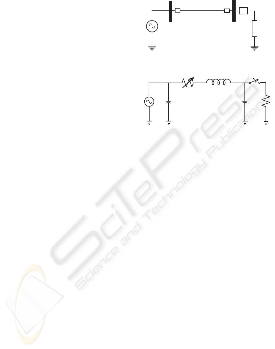
connection of the load, see Figure 3(a).
The disconnection of the load is equivalent to apply
an inverted step excitation.
The equipment used was an experimental console
LabVolt with an AC source of 20 volts; for captur-
ing the transient data we used the acquisition card of
National Instruments NI PCI 5112, (100 MHz, 100
MS/s 8-Bit Digitizer). The model used in this test is
the π model of the transmission line, this single-phase
transmission line is shown in Figure 3(b). The val-
ues for the elements of this model were; V s = 20v,
C
1
= 1.017µF, C
2
= 0.967µF, L = 29.65mH, and
R varies as shown in Equation (8).
R (t) = 0.0415t + 0.386 (8)
Switch
Load
Vs
C1
R
L
C2
Load
a)
b)
Vs
Figure 3: a) Single-phase transmission line, b) Equivalent
circuit.
We used these laboratory devices to simulate a
transmission line exhibiting the effects of aging.
Every two seconds R was adjusted (simulated by
a variable resistor), the transmission line was pow-
ered, and the load disconnected for four cycles (ap-
prox 70 msec). The disconnection transient effect was
recorded. This experiment takes 21 seconds approx-
imately, during which the transient response corre-
sponding to each desconexion of the load is captured.
During the experiments, the transient was recorded by
measuring the voltage in C
2
.
During data acquisition in an experiment, data are
not generally in good shape to be processed, and
therefore it becomes necessary to pretreat them to
eliminate noise and other components that can affect
the identification process. The frequency of the noise
is generally bigger than the modes of the system. In
the carried out experiments, the typical range of fre-
quencies of the system was between 100 and 300 Hz,
while the noise range was above the 900 Hz. If the
noise overlaps the frequencies of the system, the iden-
tification process will see it as a characteristic of the
response; this situation cannot be avoided, since there
is no way to distinguish between componentes in the
same frequency range, where some are genuine com-
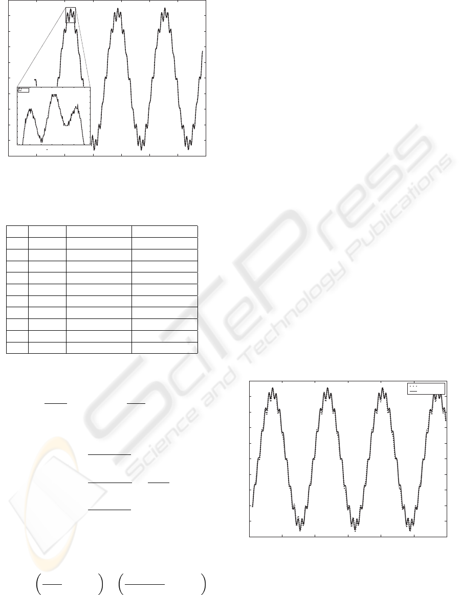
ponentes and others are noise components. Figure 4
shows the acquired signal and the detail shows the re-
sult of the filtering process.
Once the captured signals were filtered, we use the
algorithm shown in Figure 2 to process the signal. Ta-
ble 3 shows the matrix of coefficients produced by
QSI.
The π model of a transmission line expressed as an
ICINCO 2006 - SIGNAL PROCESSING, SYSTEMS MODELING AND CONTROL
58

3.92.02.012.022.03 2.04 2.05 2.06
−25
−20
−15
−10
−5
0
5
10
15
20
25
timeinseconds
magnitudeinvolts
2.01052.0112.01152.0122.0125 2.013 2.0135
18
18.5
19
19.5
20
20.5
21
21.5
22
22.5
timeinseconds
magnitudeinvolts
Filtered
Original
Figure 4: Acquired signal and detail of filtering process.
Table 3: Coefficients of a transmission line experiment.
t C
2
(t) C
1
(t) C
0
(t)
2 1 11.33780349 32147873.02
4 1 11.63152897 31834739.03
6 1 11.92525445 32076947.89
8 1 12.5127054 31982739.73
10 1 12.80643088 32087805.38
12 1 13.9813328 31982739.78
14 1 15.15623471 31955757.71
16 1 17.50603855 32018490.09
18 1 22.79309717 32087809.44
20 1 35.71701824 32018492.74
ODE is shown in equation (9)
L (t) C (t)
d
2
v
c
2
dt
2
+ R (t) C (t)
dv
c
2
dt
+ v
c
2
= v
s
(9)
therefore
C
2
(t) =
L (t) C (t)
L (t) C (t)
= 1 (10)
C
1
(t) =
R (t) C (t)
L (t) C (t)
=
R (t)
L (t)
(11)
C
0
(t) =
1
L (t) C (t)
(12)
The genetic algorithm must determine the func-
tions for R (t), L (t) and C (t) in such a way that
Equation (13) is minimized.
dif (t) =
R (t)
L (t)
− C
1
(t)
+
1
L (t) C (t)
− C
0
(t)
(13)
Following the procedure described in section 4, the
genetic algorithm first tests fitness with second degree
polynomials. As the approach provided by the second
degree polynomials is not enough to give a good fit
to the data the algorithm tests with a polynomials of
different degree, the degree
is increased until the fitness criteria is met. This
process is carried out repeatedly until achieving a
good fit.
The polynomials that best describe the behavior of
the data of Table 3 are the following:
R (t) = 0.000474t
4
− 0.006177t
3
+ · · · (14)
+0.026557t
2
− 0.02843t + 0.268339
L(t) = −0.0000001t
4
− 0.0000003t
3
+ · · · (15)
+0.0000002t
2
− 0.0000574t + 0.0232831
C(t) = −0.000015x10
−6
t
4
+ 0.0004x10
−6
t
3
− · · ·(16)
−0.003x10
−6
t
2
+ 0.01x10
−6
t + 1.33x10
−6
As we can observe in the functions given by Equa-
tions (15) and (16), the coefficients of the terms from
the first to the fourth order are small compared to the
independent term.
That is to say, these terms do not contribute signif-
icantly in the evaluation of their respective functions.
In practical terms we can assume that those functions
are constant.
Figure 5 shows the signal observed in a frozen-
instant, k, and their corresponding simulated signal
after the identification process. We compute the coef-
ficients using Equations (14), (15), and (16) evaluated
at instant k.
8.08.018.028.03 8.04 8.05 8.06
−25
−20
−15
−10
−5
0
5
10
15
20
25
time
voltage
yobserved
yestimated
Figure 5: Comparing between observed response and esti-
mated model response.
The correlation coefficient between the model es-
timated and the expected model is r = 0.9988. i.e.,
the model that we estimate reproduces the dynamics
of the system appropriately.
IDENTIFICATION OF SLOWLY TIME-VARYING SYSTEMS BASED ON THE QUALITATIVE FEATURES OF
TRANSIENT RESPONSE A FROZEN-TIME APPROACH
59

6 CONCLUSIONS
In this paper, a new identification algorithm for slowly
time-varying systems has been proposed. The algo-
rithm is based on the QSI and frozen-time approaches.
We pretreated the signal using a low-pass filter to
eliminate the inherent noise to the laboratory mea-
surements. The example of aplication of this method
was satisfactory, since the model can reproduce the
dynamics of the system with great accuracy. The al-
gorithm has been extensively tested with synthetic ex-
amples (i.e. simulations) using matlab and simulink,
and also with real laboratory measurements. The val-
idation tests of the estimated models are acceptable,
with correlation coefficients very near to unity.
ACKNOWLEDGEMENTS
The present work has been developed while Juan J.
Flores was on sabbatical at the University of Oregon.
He thanks the U of O for all the resources and accom-
modations that made his stay at the U of O and this
work possible.
REFERENCES
C. A. Desoer. ”Slowly varying discrete systems x
i+1
=
A
i
x
i
,” Electronics Letters 6, pp. 339-340, 1970.
J.E. Dennis Jr. and Schnabel Robert B. ”Numerical Methods
for Uncostrained Optimization and Nonlinear Equa-
tions”. Classics in Applied Mathematics. SIAM. 2000.
Flores Juan and Pastor Nelio. ”Qualitative and Quantitative
Systems Identification for Linear Time Invariant Dy-
namic Systems”, Workshop on Qualitative Reasoning
2002 Sitges Barcelona Espa
˜
na. Junio 2002.
Pohlheim Hartmut. “”Evolutionary Algorithms: Princi-
ples, Methods and Algorithms”” , document part of
the Genetic and Evolutionary Algorithm Toolbox for
use with MatLab. http://www.geatbx.com. November
2001.
Le Yi Wang. ”Identification and Control of Slowly Varying
Systems: Recent Advances”; Proceedings of the 34th
Conferece on decision & control, New Orleans, LA
December 1995.
Lenart Ljung. ”System Identification: Theory for the user”,
2nd Edition Upper Saddle River, NJ: Prentice Hall
1999.
M. Freedman and G. Zames. ”Logarithmic variation crite-
ria for stability of systems with time-varying gains”,
SIAM J. Control vol. 6,N
◦
3. pp. 487- 507. 1968.
Mahmood Samavat and Ali Jabar Rashidie. ”A new Algo-
rithm for Analisys and Identification of Time Varying
Systems”, Proceedings of the American Control Con-
ference, Seattle Washington, June 1995
M
¨
uhlenbein H. Schlierkamp-Voosen D., ”Predictive Mod-
els for the Breeder Genetic Algorithm: I. Continuos
Parameter Optimization”, Evolutionary Computation
1(1):25-49, 1993.
Pastor G. Nelio. ”Identificaci
´
on de Sistemas Usando Algo-
ritmos Gen
´
eticos”, Masters Thesis. Facultad de In-
genier
´
ıa El
´
ectrica, Universidad Michoacana de San
Nicol
´
as de Hidalgo, Morelia, M
´
exico. 2000.
Pastor G. Nelio. ”Identificaci
´
on de Sistemas Din
´
amicos
Variantes e Invariantes en el Tiempo Basada en las
Caracter
´
ısticas Cualitativas de la Respuesta Tran-
sitoria”, Doctoral Thesis. Facultad de Ingenier
´
ıa
El
´
ectrica, Universidad Michoacana de San Nicol
´
as de
Hidalgo, Morelia, M
´
exico. 2005.
Flores R. Juan and Pastor G. Nelio. ”Time-Invariant Dy-
namic Systems Identification Based on the Qualita-
tive Features of the Response”. Engineering Appli-
cations of Artificial Intelligence Volume 18, Issue 6,
Pages 719-729. doi:10.1016/j.engappai.2005.01.003
September 2005.
Smith Steven W. ”The Scientist and Engineer’s Guide to
Digital Signal Processing”, Second Edition, Califor-
nia Technical Publishing, San Diego California 1999.
ICINCO 2006 - SIGNAL PROCESSING, SYSTEMS MODELING AND CONTROL
60