THE HIERARCHICAL MAP FORMING MODEL

Luis Eduardo Rodriguez Soto

National Taiwan University

Taipei, Taiwan

Cheng-Yuan Liou

National Taiwan University

Taipei, Taiwan

Keywords:

Self-Organizing Maps, Q-learning, Hierarchical Control.

Abstract:

In the present paper we propose a motor control model inspired by organizational priciples of the cerebral

cortex. Speciﬁcally the model is based on cortical maps and functional hierarchy in sensory and motor areas

of the brain. Self-Organizing Maps (SOM) have proven to be useful in modeling cortical topological maps

(Palakal et al., 1995). A hierarchical SOM provides a natural way to extract hierarchical information from the

environment, which we propose may in turn be used to select actions hierarchically. We use a neighborhood

update version of the Q-learning algorithm, so the ﬁnal model maps a continuous input space to a continuous

action space in a hierarchical, topology preserving manner. The model is called the Hierarchical Map Forming

model (HMF) due to the way in which it forms maps in both the input and output spaces in a hierarchical

manner.

1 INTRODUCTION

1.1 Cerebellar Organization

Modular organization is the norm in the cerebral cor-

tex, which is divided into speciﬁc dedicated areas. For

example, there are areas dedicated to visual process-

ing, auditory signal processing and somato-sensory

processing (Muakkassa and Strick, 1979; Palakal et

al., 1995). These speciﬁc dedicated areas within the

cortex are referred to as cortical maps. Another or-

ganizational principle in the cerebral cortex is hier-

archical processing, most vastly studied in the visual

regions. Areas dedicated to motor commands have

also been shown to be organized in a hierarchical

manner. This organization in the brain is not genet-

ically pre-deﬁned and may come about through self-

organizing principles. Our work is also inspired by

the work of (Wolpert and Kawato, 1998) and their

modular selection and identiﬁcation for control (MO-

SAIC) model The MOSAIC model is based on mul-

tiple pairs of forward (predictor) and inverse (con-

troller) models. Their architecture learns both the in-

verse models necessary for control as well as how to

select the set of inverse models appropriate for a spe-

ciﬁc environment. Learning in the architecture, origi-

nally driven by the gradient-descent method, has been

later implemented by other learning methods such as

expectation-maximization (EM) algorithm, and other

reinforcement learning methods. Their model is mo-

tivated by human psychophysical data, from which

it is known that an action selection process must be

driven by two different processes: a feedforward se-

lection based on sensory signals, and selection based

on the feedback of the outcome of a movement. The

basic idea behind the MOSAIC model, is that the

brain contains multiple pairs of forward (predictor)

and inverse (controller) models wich are tightly cou-

pled during both learning and use. We studied the

MOSAIC model and wanted to produce a a similar

model but one which acquires the relation between

predictors and controllers through self-organisation

principles, in order to reﬂect the existence of the brain

maps found in the cortex. Our model combines two

different learning techniques to imitate the organized

structure of the brain, with the purpose of producing

a biologically plausible control algorithm. The cur-

rent work is a work a progress, and the results pre-

sented here are from preliminary tests, and involved

the learning of actions, mapping from an input space

to an output space. Further testing will measure the

robustness of the system described in motor control

tasks.

167

Eduardo Rodriguez Soto L. and Liou C. (2006).

THE HIERARCHICAL MAP FORMING MODEL.

In Proceedings of the Third International Conference on Informatics in Control, Automation and Robotics, pages 167-172

DOI: 10.5220/0001221801670172

 SciTePress

Layer 2

Layer 1

Layer 3

Layer 0

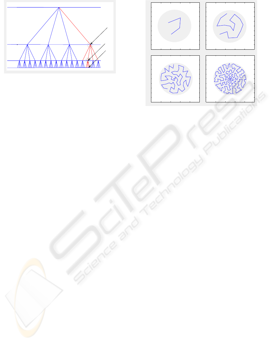
Figure 1: TSSOM with 4 layers and bf = 4.

1.2 Tree-Structured Self-Organizing

Maps

The Self-Organizing Map (SOM) was ﬁrst introduced

by Teuvo Kohonen in 1981. A hierarchical SOM

called the Tree-Structured SOM (TS-SOM) was intro-

duced by Koikkalainen and Oja (1990), and extended

in Oja and Kaski (1999). Given that there is a vast

amount of publications regarding the SOM (Kohonen,

1998, 2001; Oja and Kaski, 1999) we do not present

the mathematical detail for it in this paper. Instead we

present the dynamics of the TS-SOM which we use

as part of our model.

1.2.1 Detail of TS-SOM

The TS-SOM (Oja et al., 1999) is composed of sev-

eral layers, where each layer of the tree is a standard

SOM (Kohonen, 2001). Every node not in the ﬁnal

layer has bf child neurons in the layer below, where

bf is the branching factor. Layers are labeled in in-

creasing order, begining with a root layer or layer 0

as shown in Figure 1. Each layer l also represents

an SOM denoted M

and a neuron i in this layer can

be denoted by M

(i). Each layer l will then contain

= (bf)

neurons.

The child neuron j of neuron i in layer l will be de-

noted in the following manner: C

(j) where j ∈

{1, .., bf}; neuron j can only belong to layer l + 1,

therefore C

(j) = M

l+1

(j).

Training the TS-SOM TS-SOM is trained in a

layer by layer manner with the ﬁrst layer trained no

differently than a standard SOM. In the remaining

layers only a subset of neurons are selected to com-

pete for a given input. When an input vector U (t) is

received at time t, neurons in the ﬁrst layer all com-

pete, and a winner M

(∗) is selected. The winner se-

lects its neighbors deﬁned by a time varying neighbor-

hood function, N (t).Only the child neurons of these

0 0.2 0.4 0.6 0.8 1

0.1

0.2

0.3

0.4

0.5

0.6

0.7

0.8

0.9

0 0.2 0.4 0.6 0.8 1

0.1

0.2

0.3

0.4

0.5

0.6

0.7

0.8

0.9

0 0.2 0.4 0.6 0.8 1

0.1

0.2

0.3

0.4

0.5

0.6

0.7

0.8

0.9

0 0.2 0.4 0.6 0.8 1

0.1

0.2

0.3

0.4

0.5

0.6

0.7

0.8

0.9

Layer 1 Layer 2

Layer 3 Layer 4

Figure 2: TS-SOM with a branching factorof 4 and 4 layers.

selected neurons are allowed to compete for the input

in the next layer. This dynamic of selecting only the

children of the winning neuron and its

neighbors for competition reduces the search space

greatly (Oja et al, 1999). The neighborhood function

is also used during the updating phase, or the coop-

erative phase, in which the neighbors of the winning

neurons are allowed to update their weights towards

the current input.

Pseudo-code algorithm The dynamics of the TS-

SOM may be more clearly understod by following the

steps of the pseudo-code algorithm:

TS-SOM

Initialize

for CurrentLayer = 1 to L

while(not converged)

for i = 1 to CurrentLayer - 1

compete(C

∗

i−1

, U(t))

(∗) = winner(C

∗

i−1

)

update(M

(∗), N(t))

end

end while

end for

The update and compete subroutines behave as de-

ﬁned for the standard SOM (Kohonen, 2001; ). We

deﬁne a small number ǫ as our convergence criterion

which is calculated recursively in the following man-

ner:

= κǫ

t−1

+ ||w

− w

t−1

ICINCO 2006 - INTELLIGENT CONTROL SYSTEMS AND OPTIMIZATION

168

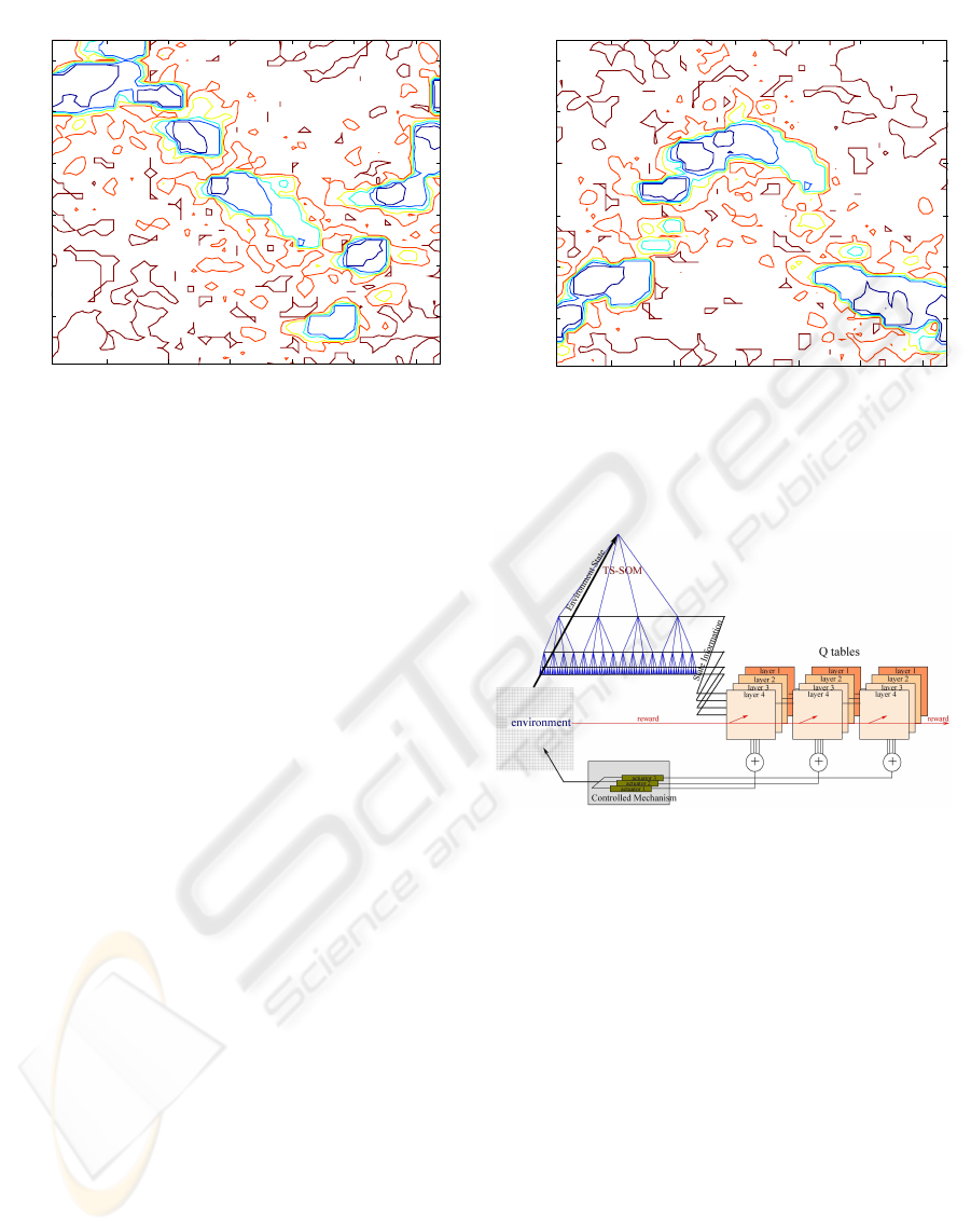
Q-table Contour Map Actuator 1

State TS-SOM

Actuator 1 Action

10 20 30 40 50 60

Figure 3: Q-value contour for actuator 1.

The term ||w

− w

t−1

|| represents the absolute value

of variation in the winning neuron’s weights after the

last update, and κdenotes a discount factor. We use

κ = 0.25 in the simulations presented in this paper.

Once ǫ is very small, for example ǫ ≤ 0.0025 we stop

the training.

In Figure 2 we see a trained 4 layer TS-SOM with bf

= 4. The TS-SOM is trained with a circular homo-

geneous density surface depicted by the shaded circle

in Figure 2. With each increasing layer, the TS-SOM

spreads more evenly over the input area, thus better

approximating the input space. In control applications

this property is very desirable, since we may abstract

higher dimensional input spaces to a 1 dimensional

space.

Thus the TS-SOM is utilized in the HMF model

to abstract higher dimensional spaces to hierarchical,

lower dimensional ones. The winning neurons of the

TS-SOM will conform the state vector, characterizing

the current state of the environment.

2 THE HMF MODEL

The HMF model applies Q-learning (Sutton and

Barto; 1998, Haykin, 1999; Watkins and Dayan,

1992) in order to map input vectors to actions. Af-

ter the TS-SOM has converged, it observes the en-

vironment as depicted in Figure 3. Each full it-

eration of the converged TS-SOM selects one win-

ning neuron per layer, forming a state vector

X =

(∗), M

(∗), ..., M

(∗)]. This state information is

fed into a group of Q-tables, where each group con-

Q-table Contour Map Actuator 2

State TS-SOM

Actuator 2 Action

10 20 30 40 50 60

Figure 4: Q-value contour for actuator 2.

Figure 5: HMF model diagram. Combines TSSOM and Q-

learning.

trols one actuator (Figure 5). The Q-tables then select,

independenty, the highest valued actions in a hierar-

chical manner as each table receives more detailed

information about the current state, or select a ran-

dom action with a probability given by ε(t) which

decreases with time. The selected actions are added,

and fed to the actuators as in Figure 5. If there are L

layers in the TS-SOM we will have L corresponding

Q-tables per actuator. Each higher indexed table will

produce higher deﬁned actions. The range of actions

per table is left to the designer to decide.

Depending on the outcome of the action selected

by the Q-tables, the enviroment will react and give a

reward signal, which is fedback to all groups of Q-

tables. The use of Q-learning for the HMF model

was motivated by the possibility that motor learning

in humans may be driven by a form of reinforcement

THE HIERARCHICAL MAP FORMING MODEL

169

TS-SOM State

Actuator 1 Action

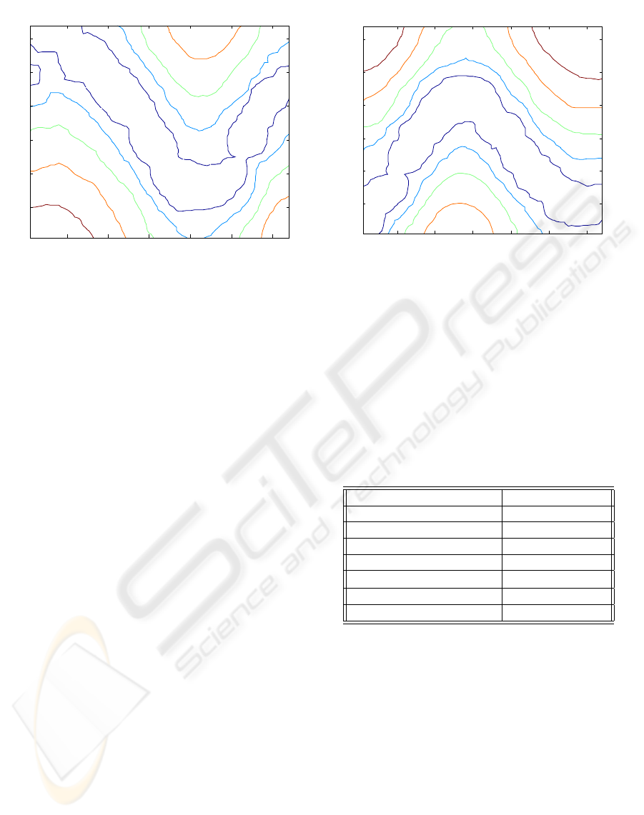
Q-values Contour Map Actuator 1

10 20 30 40 50 60

-0.1

-0.2

-0.3

-0.4

-0.5

-0.1

-0.2

-0.3

-0.4

Figure 6: NQ-value contour for actuator 1.

signal (Holroyd and Coles, 2002). As in standard Q-

learning the selection of an accurate reward signal is

essential to assure the system will properly learn the

task at hand.

2.1 Neighborhood Q-learning

In the present model we use a version of Neighbor-

hood Q-learning, where the update rule for the Q-

tables is given by:

Q(s

, a

) ← Q(s

, a

) + α ∗ η (t) ∗ [r

+ 1 +

γ max

Q(s

t+1

, a) − Q(s

, a

)]

Where the parameter α is the learning rate, and r

is the reward received at the current time t; γ is

the discount factor. The term η(t) denotes the Q-

neighborhood, and it is a time decreasing function.

Similar neighborhood Q-learning functions have been

proposed in Smith (2001), and in Millan et al. (2002).

This forms the core of the HMF model, amodel which

is currently still under development. To show the ad-

vantages of using the HMF model for action control

tasks we setup a simulated environment. We use a

mechanism as that shown in Figure 8, where the base

does not move, it is only allowed to move 2 joints.

The task is to follow a dot in a circular motion, as pre-

sented in Smith (2001). In Figure 8 we also show the

last layer of our converged TS-SOM, which closely

ﬁts the circular motion, in a topology preserving man-

ner. On each step a reward will be given equal to the

negative of the distance from the present input, plus

the radius of the sensor (r= 0.05). Thus, if the input

TS-SOM State

Actuator 2 Action

Q-Values Contour Map Actuator 2

10 20 30 40 50 60

-0.2

-0.1

-0.3

-0.4

-0.5

-0.4

-0.3

-0.2

-0.1

Figure 7: NQ-value contour for actuator 2.

data is inside the sensor a positive reward is given. We

divide the training of the HMF model in two periods,

one to learn to appropriate values for the TS-SOM,

and the second period to learn to match the input to

appropriate actions. We train our HMF model with

the parameters shown in Table 1.

Table 1: Parameters used during training.

TS-SOM size 6 layers, bf =2

Learning Rate 0.25

Initial Q-Neighborhood 20

Q-table Size 64 x 64

Training Steps 50000

Annealing Schedule e

−t/2000

Angle Range Actuator 1 0 - 1.6 radians

Angle Range Actuator 2 1.5 - 3.5 radians

The training is done over 50000 steps, following the

example set by Smith (2001), and the training is re-

peated 20 times. In Figure 9 we can see the per-

formance curve of our model contrasted to neighbor-

hood, and standard Q-learning averaged over the 20

simulations. After 20000 steps the average reward

has been maximized. Using neighborhood Q-learning

our HMF model receives higher rewards than stan-

dard Q-learning after convergence has been achieved,

but not higher than a single table neighborhood Q-

learning. While the hierarchical selection of actions

does not provide higher rewards, it does fare better

than standard Q-learning. Also, the use of hierarchi-

cal selection of actions explores the state space in a

more orderly fashion, in contrast to just selecting ran-

dom actions over a long period of time. This ordered

ICINCO 2006 - INTELLIGENT CONTROL SYSTEMS AND OPTIMIZATION

170

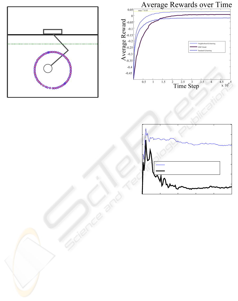
Figure 8: Simple 2 DOF mechanism used for action learn-

ing. The last converged layer of the TS-SOM is also shown.

exploration of the state space makes our model more

suitable for real world action learning tasks. In Figure

10. we compare the standard deviation, σ, of both Q-

learning update rules. The neighborhood Q-learning

minimizes the σ over time, thus beign more suitable

for stable control tasks, while in standard Q-learning

σ remains large throughout.

The Neighborhood Q-learning update rule also pre-

serves the topology in the action space. Since the

state vector

X, is received from the layers of the TS-

SOM, the states are topological neighbors in the in-

put space and in index number. Thus we expect that

actions should also be topologically similar in the Q-

table. That is the actions selected for neighbors in the

input space should be close to each other in the out-

put space. The use of the neighborhood Q-learning

ensures this as rewards are shared among neighbors

in the Q-table, thus actions close to each other in the

Q-table have similar values.

Figures 6 and 7 we see a contour mapping of a

single neighborhood Q-table. We may contrast these

contour plots to Figures 3 and 4 which are the contour

plots for Q-tables trained with the standard Q-learning

update rule. As we can see neghborhood Q-learning

maitains a topological relatioship across the table. In

Figures 3 and 4 we see that the actions values are not

similar between adjacent states, thus the mechanism

will only move in jerky motions. The training with

the neighborhood update rule produces smoothly out-

lined contours even during the early stages of training

due to the large initial neighborhood. In future imple-

mentations, currently under development and testing,

we will extend the model to allow a mapping to a con-

tinuous action range by using a softmax function as

that used in Millan et al. (2002).

Figure 9: Rewards received averaged over 20 simulations.

0 1 2 3 4 5

x 10

0.002

0.004

0.006

0.008

0.01

0.012

0.014

Time Step

Standard Deviation

Standard Deviation over Time

Standard Q-learning

Neighborhood Q-learning

Figure 10: Comparison of the Standard Deviation.

3 CONCLUSIONS

The HMF model presented here is a work in progress.

In the initial experiments it has shown to be very ef-

ﬁcient at learning the intrinsic hierarchy of the task at

hand. Extracting the state information in a hierarchi-

cal manner allows the controller portion of the model

to react hierarchically. The use of the Neighborhood

Q-learning update rule greatly enhances learning, al-

lowing the model to learn a smooth mapping to the

state information. The use of the neighborhood up-

date rule also reduces the variance of the rewards re-

ceived over time, allowing for a more stable learning

curve, this is a desirable property for real life applica-

tions, since we can be more certain how the learning

system will behave under controlled conditions. The

THE HIERARCHICAL MAP FORMING MODEL

171

mapping in the output space is done in a topology pre-

serving fashion which produces smooth movements,

even at the earlier stages of learning, which allows for

quicker learning. Work is still needed to measure the

robustness of the learning system when trained under

the effect of disturbances. Future work envisions the

extension of this model from a discrete model to a

continuous one.

REFERENCES

Holroyd, C.B. Coles, M. (2002). The Neural Basis of

Human Error Processing: Reinforcement Learning,

Dopamine, and the Error-Related Negativity Psycho-

logical Review. Vol. 109, No. 4, 679–709.

Kohonen, T. (2001). Self-Organizing Maps. Springer Ver-

lag, Heidelberg, Germany.

Koikkalainen, P. and Oja, E. (1990). Self-organizing hierar-

chical feature maps. In Proceedings of International

Joint Conference on Neural Networks (IJCNN’90) In-

formation Systems.

Millan , J. Possenato, D. Dedieu, E. (2002). Continuous-

Action Q-Learning. Machine Learning. Springer,

Netherlands .

Muakkassa, K. F., Strick, P. L. (1979). Frontal Lobe Inputs

to Primate Motor Cortex. Evidence for Four Soma-

totopically Organized ”Premotor” Areas. Brain Re-

search. Elsevier/North-Holland Biomedical Press.

Oja, E. and Kaski ,S. (1979). Kohonen Maps. Elsevier

Science, Netherlands.

Palakal, M.J. Murthy, U. Chittajallu, S.K. Wong, D. (1995).

Tonotopic Representation of Auditory Responses Us-

ing Self-Organizing Maps. Mathematical and Com-

puter Modelling. Elsevier Science, Netherlands.

Smith, A.J. (2001). Applications of the self-organising map

to reinforcement learning. Neural Networks. Elsevier,

United States

Simon Haykin. (1999). Neural Networks. Prentice-Hall,

New Jersey, Second Edition.

Watkins,C. Dayan,C. (1992). Technical Note: Q-Learning.

Machine Learning. Springer, Netherlands.

Wolpert, D. Kawato, M. (1998). Multiple Paired Forward

and Inverse Models for Motor Control. Neural Net-

works. Elsevier, United States

ICINCO 2006 - INTELLIGENT CONTROL SYSTEMS AND OPTIMIZATION

172