
Coordinated Transportation of a Large Object by a
Team of Three Robots
Rui Soares
1
and Estela Bicho
2
1
Esc. Sup. Tec. e Gest
˜
ao de Felgueiras - Instituto Politecnico do Porto, Portugal
2 ⋆⋆
Dep. Electr
´
onica Industrial, Universidade do Minho, Portugal
Abstract. Dynamical systems theory in this work is used as a theoretical lan-
guage and tool to design a distributed control architecture for a team of three
robots that must transport a large object and simultaneously avoid collisions with
either static or dynamic obstacles. The robots have no prior knowledge of the
environment. The dynamics of behavior is defined over a state space of behav-
ior variables, heading direction and path velocity. Task constraints are modeled
as attractors (i.e. asymptotic stable states) of the behavioral dynamics. For each
robot, these attractors are combined into a vector field that governs the behavior.
By design the parameters are tuned so that the behavioral variables are always
very close to the corresponding attractors. Thus the behavior of each robot is
controlled by a time series of asymptotical stable states. Computer simulations
support the validity of the dynamical model architecture.
1 Introduction
The challenge to develop teams of autonomous robots that are able to transport large
objects is an important endeavor since such multi-robot teams would be potentially
useful in many fields related to our daily activities (e.g. [1,2,4, 9, 10]).
From the point of view of a robot, the environment, which comprises the others
robots and the world scenario, exhibits complex dynamic behavior. The problem is
exacerbated when the environment is not known and no path is given. If motion coor-
dination of two robots carrying an object is not a trivial task, motion coordination of
larger teams is undoubtedly more difficult.
Here we present results on the problem of coordinating and controlling three mobile
robots that must carry a rigid object from an initial position to a final target destination.
This paper extends previous work reported in [6, 8]. In those works dynamical sys-
tems theory was used as the theoretical framework to design and implement a distrib-
uted control architecture for a team of two mobile robots that cooperatively had to
transport a long object in a cluttered environments.
Here it is assumed that: (a) the robots have no prior knowledge of the environment
and no path is given; (b) a leader-helper decentralized motion control strategy is used,
where the leader robot moves from an initial position to a final target destination (see
⋆⋆
corresponding author
Soares R. and Bicho E. (2006).
Coordinated Transportation of a Large Object by a Team of Three Robots.
In Proceedings of the 2nd International Workshop on Multi-Agent Robotic Systems, pages 66-79
DOI: 10.5220/0001222600660079
Copyright
c
SciTePress

e.g. [9]); (c) each helper robot (H
1
and H
2
) takes the leader and the other helper robot
as reference points and must maintain at all times a correct distance and orientation
with them that permits it to help them in the transportation task (see Figure 1).
forward/backward
formation
target
leader
H
1
H
2
turn
formation
column
formation
turn
formation
obstacle
forward/backward
formation
Fig.1. Coordinated object transportation by three robots in an unknown environment. By de-
fault the robots must transport the object keeping a forward/backward formation (f/b). When due
to encountered obstacles that is not possible the helper robots must drive in turn or in column
formation.
The control architecture of each robot is structured in terms of elementary behav-
iors. The individual behaviors and their integration are generated by non-linear dynami-
cal systems. For each behavior, desired values for the controlled variables are identified
and made attractor solutions of the dynamical systems that generates the robots’ motion.
The rest of the paper is structured as follows: the next section presents the robot
team, their tasks and the basic assumptions in this work. The behavioral dynamics are
then defined for the robot helpers (H
1
and H
2
). Results obtained from computer simu-
lations are presented in section 4. The paper ends with a brief discussion, conclusions
and an outlook of future work.
2 Robot Team and Task Constraints
The simulated robots are based on the physical mobile robots used in [8] but the sup-
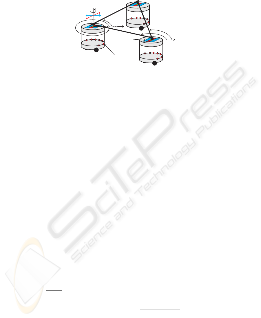
port base for the object is new. This support base gives displacements (∆x, ∆y) and
rotation (∆w) of the object (see Figure 2). The coordination and control are based on
the following ideas: (a) the behavior of each robot is controlled independently; (b) the
leader robot knows the target position, and its task consists in moving from an initial
position to a final target destination; (c) the task constraints for the helper robots consist
in keeping at all times a correct orientation and distance with respect to the leader and
the other helper; (d) by default the helpers must move in an F/B formation, however
if obstacles do not allow it, they must adequately move in turn or column formation
to guarantee obstacle avoidance for the team; (e) the leader robot broadcast it´s ve-
locity and heading direction to the helpers; (f) each helper from ∆x, ∆y and ∆w is
able to compute the directions at which the leader and the other helper lie from its cur-
rent position and with respect to an external reference axis, i.e. ψ
H
i
,leader
and ψ
H
i
,H
j
67
y
H1,leader
x
H1
leader
Distance
sensores
y
H2,leader
x
H2
y
H1,H2
y
H2,H1
Dx
Dy
Support
base
Dw
Fig.2. Each robot has seven distance sensors mounted on a ring which is centered on the robot’s
rotation axis. These are used to measure the distance to obstructions at the direction in which
they are pointing in space. The simulated infrared sensors have a distance range of 60cm and an
angular range of 30
o
. The robots are tightly coupled through a support base mounted on each
robot. It consists of two prismatic and one rotational passive joints which allow to compute the
directions at which each helper robot “sees” the leader and the other helper from its current
position, ψ
H
i
,leader
and ψ
H
i
,H
j
(i = 1, 2; j = 1, 2; i 6= j), and displacements (∆x, ∆y) and
orientation (∆w) of the object.
(i = 1, 2; j = 1, 2; i 6= j) respectively (see Figure 2); (g) the helper robots broad-
cast their heading direction values; (h) each helper broadcasts its current values of the
potential function and magnitude, of the virtual obstacles avoidance dynamics; (i) the
helper robots do not need to know the object size, they only need to know the displace-
ment and rotation of the transported object in their support base; (j) the robots have
nonholonomic motion constraints.
3 Attractor Dynamics for Coordinated Transportation
To model the robots behavior their heading direction is used, φ (0 ≤ φ ≤ 2π), with
respect to an arbitrary but fixed world axis and path velocity, ϑ. Behavior is generated
by continuously providing values to these variables, which control the robot’s wheels.
The time course of each of these variables is obtained from (constant) solutions of
dynamical systems. The attractor solutions (asymptotically stable states) dominate these
solutions by design. The leader’s heading direction and path velocity dynamics has been
previously define, implemented and evaluated in [3], but for the obstacle avoidance
dynamics the leader robot takes into account it’s size as well as the dimensions of the
team. H
i
’s (i = H
1
, H
2
) heading direction and path velocity dynamics are ruled by the
following dynamical systems:
dφ
H
i
(t)
dt
= −2λ
H
i
cos (λ
desired,H
i
) sin (φ
H
i
− ψ
desired,H
i
) + f
stoch
(1)
dϑ
H
i
(t)
dt
= −c
H
i
(ϑ
H
i
− V
desired,H
i
)e
−
(
ϑ
H
i
−V
desired,H
i
)
2
2σ
2
V
+ g
stoch
(2)
68

The heading direction dynamics (1) puts an attractor at ψ
desired,H
i
with a strength of
attraction (relaxation rate) defined by −2λ
H
i
cos (λ
desired,H
i
), and a repeller in the op-
posite direction. The path velocity dynamics (2) defines a simple attractor at the desired
path velocity with a relaxation rate defined by c
H
i
. The exponential term in (2) is used
to make sure that the increasing and decreasing of velocity is smooth even when the
difference ϑ
H
i
− V
desired,H
i
is very large. f
stoch
and g
stoch
are stochastic forces that
are added to the dynamical systems, to simulate perturbations and noise in the system.
In the next two subsections will be explained how the attractor values for heading
direction and path velocity are computed from sensed and/or communicated informa-
tion. From now on H
i
= H
1
, H
2
; H
j
= H
1
, H
2
; H
i
6= H
j
.
3.1 Attractor Dynamics for Heading Direction
The heading direction dynamics, for each helper is governed by (1) where:
ψ
desired,H
i
= γ
H
i
,f/b
ψ
desired,H
i
,f/b
+ γ
H
i
,turn
ψ
desired,H
i
,turn
+
+γ
H
i
,column
ψ
desired,H
i
,column
(3)
λ
desired,H
i
= γ
H
i
,f/b
λ
desired,H
i
,f/b
+ γ
H
i
,turn
λ
desired,H
i
,turn
+
+γ
H
i
,column
λ
desired,H
i
,column
(4)
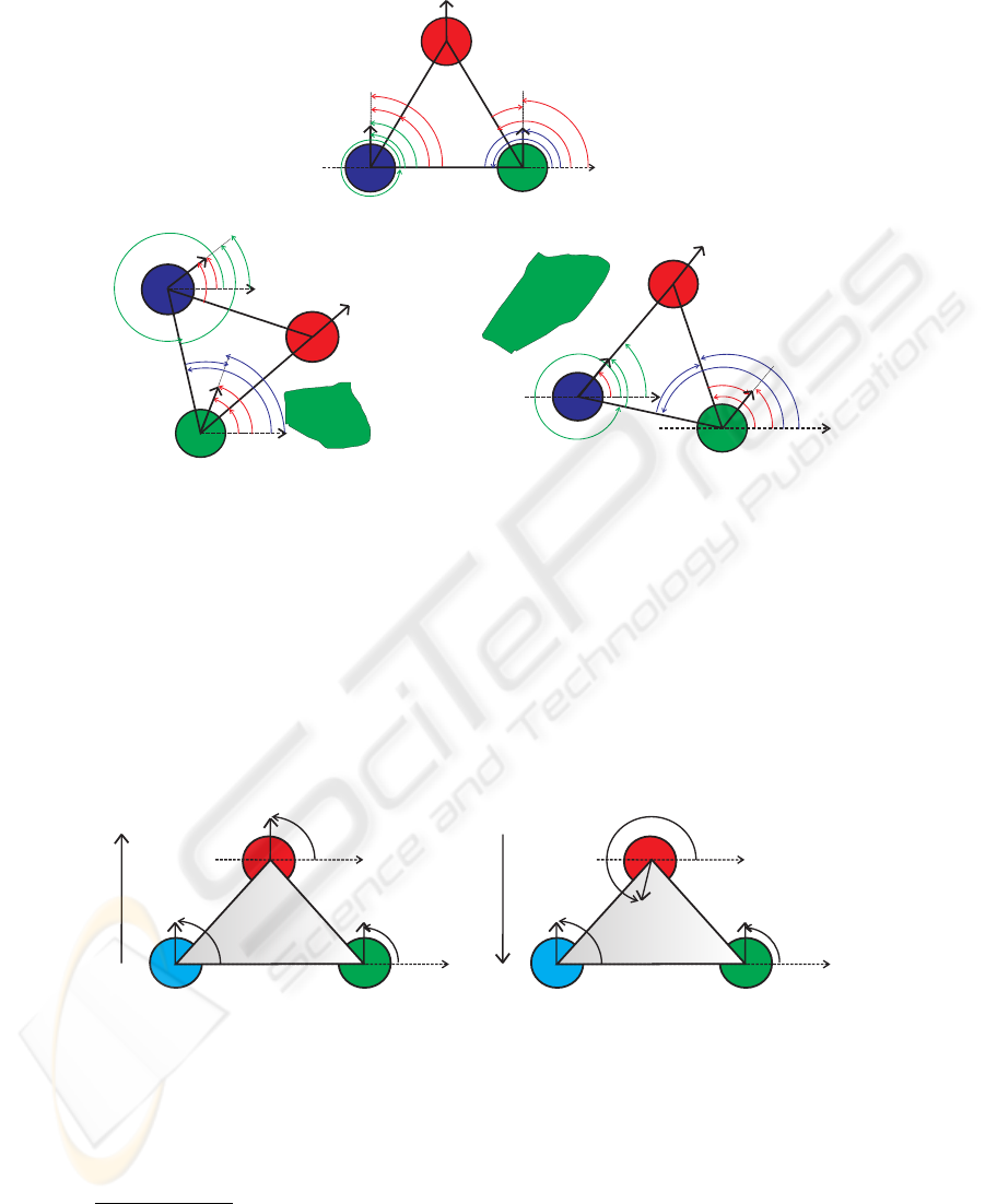
Here ψ
desired,H
i
,f/b
, ψ
desired,H
i
,turn
and ψ
desired,H
i
,column
are the desired directions
at which the attractors emerge for each different behavior, forward/backward, turn and
column formations, respectively (see Figure 3). γ
H
i
,f/b
, γ
H
i
,turn
and γ
H
i
,column
are
mutually exclusive activation variables that determine which attractor value must dom-
inate the dynamics. In the next two subsections, it will be explained how the activation
variables and the attractor values are computed from sensed and/or communicated in-
formation.
Activation Variables.
Forward/backward formation:
In the absence of obstacles robot H
i
must move in a
“f/b formation”, so the term γ
H
i
,f/b
must dominate the dynamics. Thus γ
H
i
,f/b
= 1,
γ
H
i
,turn
= 0 and γ
H
i
,column
= 0 is required.
γ
H
i
,f/b
=
+1, if α
f
i
= 1 ∨ α
b
i
= 1
0, else
(5)
where α
f
i
and α
b
i
signal the control architecture when it’s necessary for the helper
robots to move forward or backward respectively
3
(see Figure 4):
α
f
i
=
+1, if
U
obs,H
i
> 0 ∧ U
obs,H
j
> 0
∨
U
obs,H
i
≤ 0 ∧ U
obs,H
j
≤ 0
∧
|φ
H
i
− φ
leader
| < ∆θ
1
∧
φ
H
j
− φ
leader
< ∆θ
1
0, else
(6)
3
∆θ
1
is a constant. Here equal to 90
◦
69
leader
x
y
H1,leader
30º
FBformation
H
1
x
obstacle
Turnformation
x
obstacle
Columnformation
y
H1,leader,LB
y
H2,leader
y
H1,H2
90º
-30º
y
H2,leader,LB
y
H2,H1
y
H2,H1,LB
H1
H2
H2
x
y
H1,leader
60º
y
H2,leader
30º
y
H2,leader,turn
y
H1,H2
120º
y
H1,leader,turn
y
H1,H2,LB
y
H1,H2,turn
-90º
y
H2,H1,LB
-30º
y
H2,H1,turn
leader
x
leader
H
1
H2
y
H1,leader
=
y
H1,leader,turn
y
H1,H2
60º
y
H1,H2,column
-60º
y
H2,leader,column
y
H2,H1
-120º
y
H2,H1,column
Fig.3. Desired directions for each helper robot for the different behaviors.
α
b
i
=
+1, if
U
obs,H
i
> 0 ∧ U
obs,H
j
> 0
∨
U
obs,H
i
≤ 0 ∧ U
obs,H
j
≤ 0
∧
|φ
H
i
− φ
leader
| ≥ ∆θ
1
∧
φ
H
j
− φ
leader
≥ ∆θ
1
0, else
(7)
This permits robot H
i
to move forward or backward keeping a f/b formation.
leader
H
1
H
2
x
x
f
H1
f
leader
f
H2
u
H1
u
leader
u
H2
movement
direction
b)backward
leader
H
1
H
2
x
x
f
H1
f
leader
f
H2
u
H1
u
leader
u
H2
movement
direction
a)forward
Fig.4. (a) The heading direction of the leader robot isn’t pointing to a direction between the two
helper robots, the helper robots must move forward; (b) The heading direction of the leader robot
is pointing to a direction between the two helper robots, the helper robots must move backward.
Turn formation:
When obstructions are detected and the difference between the direc-
70

tion ψ
H
i
,leader
and φ
leader
is larger than a certain value, ∆θ
2
4
, we want that the robots
to move in turn formation , so the term γ
H
i
,turn
must dominate the dynamics. Thus
γ
H
i
,turn
= 1, γ
H
i
,f/b
= 0 and γ
H
i
,column
= 0. This implies robot H
i
to turn around,
i.e. avoid the obstacle by turning to the right or to the left. Robot H
i
takes this decision
based on:
α
tr
i
=
+1, if U
obs,H
i
> 0 ∧ U
obs,H
j
≤ 0 ∧ F
obs,H
i
< 0 ∧ |φ
leader
− ψ
H
i
,leader
| > ∆θ
2
0, else
(8)
α
tl
i
=
+1, if U
obs,H
i
> 0 ∧ U
obs,H
j
≤ 0 ∧ F
obs,H
i
> 0 ∧ |φ
leader
− ψ
H
i
,leader
| > ∆θ
2
0, else
(9)
where α
tr
i
and α
tl
i
signal the control architecture when it’s necessary robot H
i
to turn
right or left respectively. U
obs,H
i
and U
obs,H
j
in (8) and (9) are the potential functions
of the virtual obstacles avoidance dynamics for each helper robot, that indicate if obsta-
cles contributions are present (how to compute these see [6,8]). Positive values of these
functions indicate that the helpers heading direction are in a repulsion zone of sufficient
strength. Conversely, negative values of these functions indicates that the heading direc-
tion is outside the repulsion range or the repulsion is very weak. As shown in [6] and [8]
the virtual obstacle avoidance dynamics, F
obs,H
i
and F
obs,H
j
, can be used to signal if
obstacles are to the right or left side of robots. Positive values of these functions indicate
that an obstacle is detected at the right side of the robot. Conversely, negative values of
these functions indicate that an obstacle is detected on the left side of the robots. Finally
activation variable γ
H
i
,turn
is set by:
γ
H
i
,turn
=
+1, if α
tr
i
= 1 ∨ α
tl
i
= 1
0, else
(10)
Column formation:
If obstructions are detected and the difference between the direction
ψ
H
i
,leader
and φ
leader
is smaller than ∆θ
2
, the term γ
H
i
,column
must dominate the
dynamics, so γ
H
i
,column
= 1, γ
H
i
,f/b
= 0 and γ
H
i
,turn
= 0. This makes robot H
i
to
move in parallel with the detected obstacle, i.e. to move in right or left column. Robot
H
i
takes this decision as defined by:
α
cr
i
=
+1, if U
obs,H
i
≤ 0 ∧ U
obs,H
j
> 0 ∧ |φ
leader
− ψ
H
i
,leader
| ≤ ∆θ
2
0, else
(11)
α
cl
i
=
+1, if U
obs,H
i
> 0 ∧ U
obs,H
j
≤ 0 ∧ |φ
leader
− ψ
H
i
,leader
| ≤ ∆θ
2
0, else
(12)
where α
cr
i
and α
cl
i
signal right or left column respectively. γ
H
i
,column
can then be set:
γ
H
i
,column
=
+1, if α
cr
i
= 1 ∨ α
cl
i
= 1
0, else
(13)
4
∆θ
2
is a constant. Here equal to 5
◦
. This value is the minimal value obtained by experimental
simulations for a safe turn formation for each helper robot without losing the object.
71
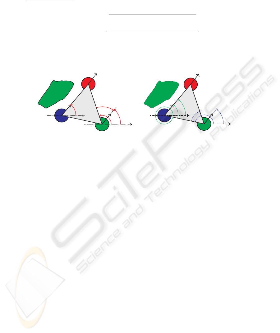
Attractor Values for Different Behaviors. From (3) it is possible to see one desired
direction for each different behavior (i.e. ψ
desired,H
i
,f/b
, ψ
desired,H
i
,turn
and
ψ
desired,H
i
,column
) (see Figure 3).
Forward/backward formation
: The desired attractor and its strengths for F/B formation
are given by:
ψ
H
i
,f/b
=
ψ
H
i
,leader,f/b
+ ψ
H
i
,H
j
,f/b
2
(14)
λ
H
i
,f/b
=
−ψ
H
i
,leader,f/b
+ ψ
H
i
,H
j
,f/b
2
(15)
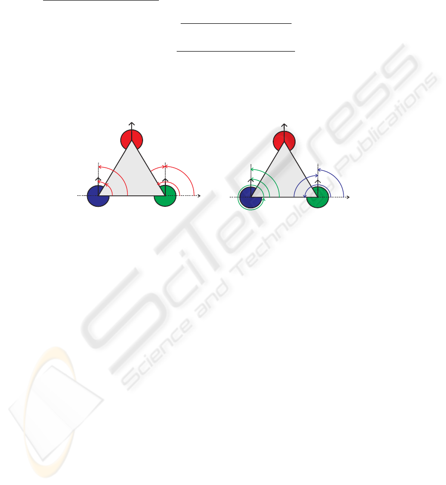
where ψ
H
i
,leader,f/b
is the desired attractor for H
i
robot with respect to the leader robot
(see Figure 5(a)) and ψ
H
i
,H
j
,f/b
is the desired attractor for H
i
robot with respect to H
j
robot (see Figure 5(b)).
leader
x
H1
H2
y
H1,leader
30º
y
H1,leader,f/b
y
H2,leader
-30º
y
H2,leader,f/b
a) b)
leader
x
y
H2,H1
H1
H2
y
H1,H2
90º
y
H1,H2,f/b
-90º
y
H2,H1,f/b
Fig.5. (a) Desired direction for each helper robot with respect to the leader robot; (b) Desired
direction for each helper robot with respect to the other. (parameters settings: k
H
1
= 1, k
H
2
=
−1, δ
f/b,H
i
,leader
= 30
◦
, δ
f/b,H
i
,H
j
= 90
◦
, R
H
1
= 1, R
H
2
= −1, ∆
H
i
= 0).
Desired direction of H
i
with respect to the leader robot: As depicted in Figure 5(a),
the attractor is set at a direction
ψ
H
i
,leader,f/b
= ψ
H
i
,leader
+ k
H
i
δ
f/b,H
i
,leader
+ R
H
i
∆
H
i
(16)
where ψ
H
i
,leader
is the direction at which H
i
robot “sees” the leader from its current
position. k
H
i
is a parameter that can take the values -1 or +1 depending on the robot
that is referred to.
k
H
i
=
+1 if H
i
= H
1
−1 if H
i
= H
2
(17)
δ
f/b,H
i
,leader
is a constant (here equal to 30
◦
). R
H
i
is a constant that can take one
of two values, -1 or +1, depending on the helper robot that is referred to and at the
parameter α
b
i
(7),
R
H
i
=
+1 if (H
i
= H
1
∧ α
b
i
= 0) ∨ (H
i
= H
2
∧ α
b
i
= 1)
−1 if (H
i
= H
1
∧ α
b
i
= 1) ∨ (H
i
= H
2
∧ α
b
i
= 0) .
(18)
72

∆
H
i
in (16), is a sigmoidal function that varies with the displacements of the object
measured by the support base, i.e. it converts the displacement of the object into an
angle that approaches null as the displacements of the object tends to zero and it is
given by:
∆
H
i
=
2 arctan (α
H
i
∆d
H
i
)
π
(19)
where α
H
i
5
is a constant and ∆d
H
i
is the displacement of the object measured by the
support base of each helper robot.
Desired direction of H
i
with respect to the H
j
robot: Figure 5(b), shows that the desired
attractor is set at a direction
ψ
H
i
,H
j
,f/b
= ψ
H
i
,H
j
+ k
H
i
δ
f/b,H
i
,H
j
+ R
H
i
∆
H
i
(20)
where k
H
i
, R
H
i
and ∆
H
i
are the same parameters used in (17), (18) and (19), respec-
tively. ψ
H
i
,H
j
is the direction at which helper H
i
“sees” helper H
j
from it´s current
position. δ
f/b,H
i
,H
j
its an angle (here equal to 90
◦
).
Turn formation
: When moving around an obstacle the desired attractor and strength for
turn formation are given by:
ψ
H
i
,turn
=
ψ
H
i
,leader,turn
+ ψ
H
i
,H
j
,turn
2
(21)
λ
H
i
,turn
=
−ψ
H
i
,leader,turn
+ ψ
H
i
,H
j
,turn
2
(22)
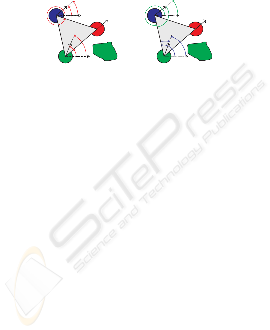
where ψ
H
i
,leader,turn
is the desired attractor of H
i
robot with respect to the leader
robot (see Figure 6(a)) and ψ
H
i
,H
j
,turn
is the desired attractor of H
i
robot with respect
to H
j
robot (see Figure 6(b)).
Desired direction of H
i
with respect to the leader robot: As it is possible to see in
Figure 6(a), the desired attractor emerges at a direction
ψ
H
i
,leader,turn
= ψ
H
i
,leader
+ δ
turn,H
i
,leader
+ R
H
i
∆
H
i
(23)
where ∆
H
i
is given by (19). R
H
i
is a parameter that takes the value 1 or -1 depending
on the helper robot are we referring to.
R
H
i
=
+1 if (H
i
= H
1
)
−1 if (H
i
= H
2
)
(24)
ψ
H
i
,leader
is the direction at which H
i
robot “sees” the leader. δ
turn,H
i
,leader
is an
angle that depends in what direction helper H
i
has to turn to, left or right.
δ
turn,H
i
,leader
=
∆ψ
H
i
,leader,turn lef t
if α
tl
i
= 1
−∆ψ
H
i
,leader,turn right
else
(25)
5
Here, α
H
1
= 0.1, α
H
2
= 1
73
x
obstacle
H2
leader
x
y
H1,leader
60º
y
H1,leader,turn
30º
y
H2,leader,turn
y
H2,leader
H
1
x
obstacle
H2
leader
x
120º
y
H1,H2,turn
y
H2,H1
y
H1,H2
-30º
y
H2,H1,turn
H
1
a) b)
Fig.6. (a)Desired direction for each helper robot with respect to the leader robot; (b) Desired
direction for each helper robot with respect to the other. (parameters settings: δ
turn,H
1
,leader
=
60
◦
, δ
turn,H
2
,leader
= 30
◦
, δ
turn,H
1
,H
2
= 120
◦
, δ
turn,H
2
,H
1
= 30
◦
, R
H
1
= 1, R
H
2
= −1,
∆
H
i
= 0).
where α
tl
i
is given by (9).
∆ψ
H
i
,leader,turn lef t
and ∆ψ
H
i
,leader,turn right
are angles that depend on what
helper robot is referred to. Here
∆ψ
H
i
,leader,turn lef t
=
60
◦
if H
i
= H
1
30
◦
if H
i
= H
2
(26)
∆ψ
H
i
,leader,turn right
=
30
◦
if H
i
= H
1
60
◦
if H
i
= H
2
(27)
Desired direction of H
i
with respect to the H
j
robot: In Figure 6(b), it’s possible to see
that the desired attractor is built at a direction
ψ
H
i
,H
j
,turn
= ψ
H
i
,H
j
+ δ
turn,H
i
,H
j
+ R
H
i
∆
H
i
(28)
where R
H
i
and ∆
H
i
are given by (24) and (19), respectively. ψ
H
i
,H
j
is the direction at
which H
i
robot sees H
j
robot. δ
turn,H
i
,H
j
it’s an angle that depends in what direction
the helper H
i
has to turn to, left or right.
δ
turn,H
i
,H
j
=
R
H
i
∆ψ
H
i
,H
j
,turn left
if α
tl
i
= 1
R
H
i
∆ψ
H
i
,H
j
,turn right
else
(29)
where α
tl
i
is given by (9). ∆ψ
H
i
,H
j
,turn left
and ∆ψ
H
i
,H
j
,turn right
are angles that
depend on what robot helper we are referring to. Here
∆ψ
H
i
,H
j
,turn left
=
120
◦
if H
i
= H
1
30
◦
if H
i
= H
2
(30)
∆ψ
H
i
,H
j
,turn right
=
30
◦
if H
i
= H
1
120
◦
if H
i
= H
2
(31)
74
Column formation: The desired attractor and strength for column formation are given
by:
ψ
H
i
,column
=
ψ
H
i
,leader,column
+ ψ
H
i
,H
j
,column
2
(32)
λ
H
i
,column
=
−ψ
H
i
,leader,column
+ ψ
H
i
,H
j
,column
2
(33)
where ψ
H
i
,leader,column
is the desired attractor of H
i
robot with respect to the leader
robot (see Figure 7(a)) and ψ
H
i
,H
j
,column
is the desired attractor of H
i
robots with
respect to each other (see Figure 7(b)).
x
obstacle
y
H2,leader
x
leader
H
1
H2
y
H1,leader
=
y
H1,leader,turn
-60º
y
H2,leader,column
x
obstacle
x
leader
H
1
H2
y
H1,H2
60º
y
H1,H2,column
y
H2,H1
-120º
y
H2,H1,column
a) b)
Fig.7. (a)Desired direction for each helper robot with respect to the leader robot; (b) Desired di-
rection for each helper robot with respect to the other. (parameters settings: δ
column,H
1
,leader
=
0
◦
, δ
column,H
2
,leader
= 60
◦
, δ
column,H
1
,H
2
= 60
◦
, δ
column,H
2
,H
1
= 120
◦
, R
H
1
= 1,
R
H
2
= −1, ∆
H
i
= 0).
Desired direction of H
i
with respect to the leader robot: As it is possible to see in
Figure 7(a), the desired attractor is built at a direction
ψ
H
i
,leader,column
= ψ
H
i
,leader
+ δ
column,H
i
,leader
+ R
H
i
∆
H
i
(34)
where R
H
i
and ∆
H
i
are given by (24) and (19), respectively. ψ
H
i
,leader
is the direction
at which H
i
robot “sees” the leader robot. δ
column,H
i
,leader
is an angle that depends on
which helper robot has to be behind the leader robot, i.e. move in column, left or right.
δ
column,H
i
,leader
=
R
H
i
∆ψ
H
i
,leader,column lef t
if α
cl
i
= 1
∆ψ
H
i
,leader,column right
else
(35)
where R
H
i
and α
cl
i
are given by (24) and (12), respectively.
∆ψ
H
i
,leader,column lef t
and ∆ψ
H
i
,leader,column right
are angles that depend on what
robot we are referring to. Here
∆ψ
H
i
,leader,column lef t
=
0
◦
if H
i
= H
1
60
◦
if H
i
= H
2
(36)
∆ψ
H
i
,leader,column right
=
60
◦
if H
i
= H
1
0
◦
if H
i
= H
2
(37)
75

Desired direction of H
i
with respect to the H
j
robot: In Figure 7(b), it is possible to
see that the desired attractor emerges at a direction
ψ
H
i
,H
j
,column
= ψ
H
i
,H
j
+ δ
column,H
i
,H
j
+ R
H
i
∆
H
i
(38)
where R
H
i
and ∆
H
i
are given by (24) and (19), respectively. ψ
H
i
,H
j
is the direction at
which H
i
robot “sees” H
j
robot. δ
turn,H
i
,H
j
is an angle that depends on which helper
has to be behind the leader robot.
δ
column,H
i
,H
j
=
R
H
i
∆ψ
H
i
,H
j
,column lef t
if α
cl
i
= 1
R
H
i
∆ψ
H
i
,H
j
,column right
else
(39)
where α
cl
i
is given by (12). ∆ψ
H
i
,H
j
,column lef t
and ∆ψ
H
i
,H
j
,column right
are angles
that depend on what helper robot we are referring to. Here
∆ψ
H
i
,H
j
,column lef t
=
60
◦
if H
i
= H
1
120
◦
if H
i
= H
2
(40)
∆ψ
H
i
,H
j
,column right
=
120
◦
if H
i
= H
1
60
◦
if H
i
= H
2
.
(41)
3.2 Attractor Dynamics for Velocity
For the leader’s path velocity control see [6]. The helpers’ path velocity must be con-
trolled so that at all times each helper robot attempts to maintain a null displacement of
the object (i.e ∆d
H
i
= 0). The leader robot communicates its current path velocity to
the helpers. The attractor value, i.e. the required velocity V
desired,H
i
, for the velocity
dynamics (2) is given by:
V
desired,H
i
=
+ϑ
leader
+
|
∆d
H
i
|
ν
H
i
, if ∆d
H
i
< 0
−ϑ
leader
−
|
∆d
H
i
|
ν
H
i
, else
(42)
∆d
H
i
is the displacement of the object measured in the support base mounted on the H
i
robot. ν
H
i
is a parameter that depends on the helper robot and on what side the helper
has to turn to.
ν
H
i
=
ν
1
, if (H
i
= H
1
∧ α
tl
i
= 1) ∨ (H
i
= H
2
∧ α
tl
i
= 0)
ν
2
else
(43)
α
tl
i
is defined by (9).ν
1
6
and ν
2
7
values were reached by simulation experiments, these
values are the minimal values obtained for a safe transportation.
3.3 Hierarchy of Relaxation Rates
The following hierarchy of relaxation rates ensures that the heading direction of each
helper relaxes to a dominant attractor solution.
c
H
i
>> 2λ
H
i
cos
λ
desired,H
i
,f/b
, c
H
i
>> 2λ
H
i
cos (λ
desired,H
i
,turn
) ,
c
H
i
>> 2λ
H
i
cos (λ
desired,H
i
,column
)
(44)
6
ν
1
is a constant. Here equal to 3.
7
ν
2
is a constant. Here equal to 9.
76
4 Results
The complete distributed dynamical architecture was evaluated in computer simula-
tions, generated by software written in MATLAB. In the simulation, the robots are rep-
resented by two Cartesian coordinates and the heading direction. Cartesian coordinates
are updated by a dead-reckoning rule, while the heading direction and path velocity
are obtained from the corresponding behavioral dynamical. All dynamic equations are
integrated with a forward Euler method with a fixed time step, and sensory information
is computed once per each cycle. Distance sensors are simulated through an algorithm
reminiscent of ray tracing. The target information is defined by a goal position in space.
It’s assumed that the leader robot communicates to the helpers its current path velocity
and heading velocity. The helper robots communicate each other their current heading
directions and its current values of the potential function and magnitude, of the virtual
obstacles avoidance dynamics.
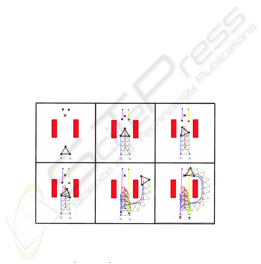
A simulation run in an environment with obstacles (static and dynamic), that demon-
strates some features of the distributed dynamic control architecture, is presented in
Figure 8. The dynamic obstacles are represented by two robots, R3 and R4. Their be-
havioral dynamics is reported in [7]. Figure 9 shows the heading direction dynamics for
each robot, at the points shown in snapshot D. We only present one simulation run and
the heading direction at one snapshot due to limitations of space (more videos can be
found in www.dei.uminho.pt/pessoas/estela/).
A
leader
H1
target
B C
D
E F
leader
H1
target
leader
H1
target
leader
H1
target
leader
H1
target
leader
H1
target
H2
H2
H2
H2
H2
H1
H2
target_R3
target_R4
R3
R4
R4
R3
target_R3
target_R4
target_R3
target_R4
target_R3
target_R4
R4
R3
R4
R3
R4
target_R3
target_R4
R3
R4
target_R3
target_R4
Fig.8. Snapshots of a simulation run the complete system. Time evolves from A to F.
In Figure 8 the targets are represented by a cross. The targets of leader, R3 and
R4 are target, target R3 and target R4, respectively. Each robot is represented by a
77
black circle with a line that represents its heading direction. Initially the robots are
placed as illustrated in Panel A. The leader moves toward its target entering in a passage
between two obstacles (Panel B), and H
1
and H
2
robots start steering forward to keep
a f/b forward formation with the leader robot. Robots R3 and R4 enter in the same
passage to reach their targets, i.e. target
R3 and target R4, respectively. Then the leader
robot detects these robots (Panel C). This forces the leader to turn back and to change
its course to avoid collisions with R3 and R4. H
1
and H
2
maintain a f/b backward
formation with the leader robot while driving backwards in the passage. The other
two robots continue moving in the direction of their targets. The leader robot continues
trying to leave the passage (Panel D) and the helpers maintain a f/b backward formation.
The robots team leaves then the passage and find a new way in the target direction
(Panel E). Robots H
1
and H
2
maintain a turn formation with the leader. Finally all
robots reach their targets (Panel F).
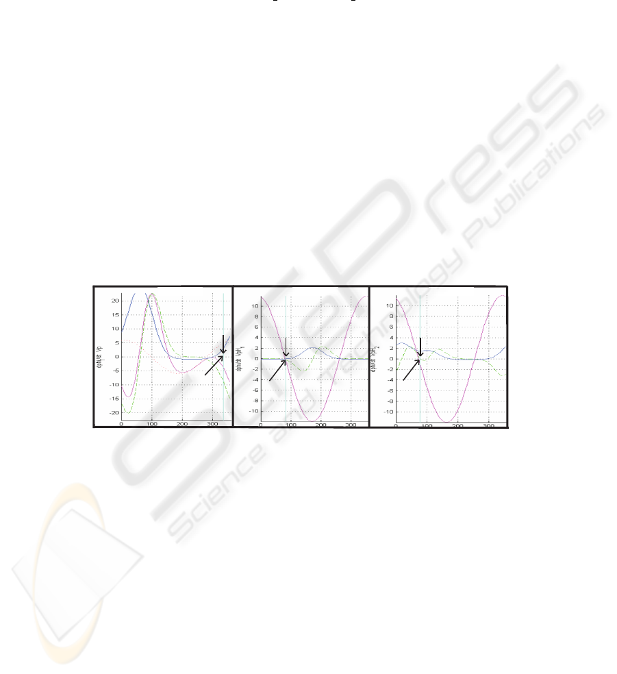
The heading directions dynamics for the three robots in the team can be seen in
Figure 9 at the position depicted at snapshot D. The black arrow in each plot indicates
the current state (i.e. heading direction in the world) of the corresponding robot. As it’s
possible to see, the heading direction of each robot is always very close to a fixed point
attractor (i.e. in the Figure 9 is the one with negative slope) of the resultant dynamics.
f
leader
g
H1,f/b
f
target,leader
U
obs,leader
f
obs,leader
U
obs,H1
f
obs,H1
U
obs,H1
f
obs,H1
D
g
H2,f/b
attractor
attractor
attractor
-active
-active
f
H1,f/b
f
H2,f/b
current
heading
direction
leader
H1:f/b-backward H2:f/b-backward
current
heading
direction
current
heading
direction
Fig.9. Heading direction dynamics for the three robots in the team when they are at positions
depicted in Figure 8. Left plot: it’s possible to see contributions of sensed obstacles (f
obs,leader
)
and target contribution (f
target,leader
). The resultant dynamics is f
leader
. Middle plot: here the
robot senses obstructions. Its heading direction is inside the repulsive range and the difference
between the H
1
robot heading direction and the heading direction of the leader robot is greater
than 90
o
, and also the difference between the H
2
robot heading direction and the heading direc-
tion of the leader robot is greater than 90
o
. Thus the resultant dynamics is dominated by the term
γ
H
1
,f/b
. Right plot: this robot also senses obstructions. Its heading direction is inside the repul-
sive range and the difference between the H
2
robot heading direction and the heading direction
of the leader robot is greater than 90
o
, and also the difference between the H
1
robot heading
direction and the heading direction of the leader robot is greater than 90
o
. Thus the resultant
dynamics is dominated by the term γ
H
2
,f/b
.
78

5 Conclusions and Future Work
In this paper, non-linear attractor dynamics was used as a tool to design a distributed
control architecture that enables a team of three robots to transport a large object. It was
assumed that the robots have no prior knowledge of the environment. The choice of the
control variables and parameters have taken into account the physical mobile robots at
which the architecture will be implemented. The amount of information communicated
among robots is minimal. The overall control system is flexible, since planning solu-
tions may change based on changes in sensed world and/or communicated information.
The leader broadcast its heading direction and path velocity (codified in 2 bytes) and
each helper share among them 3 values represented by 3 bytes. The control architec-
ture was evaluated through computer simulations. The global behavior is stable and
trajectories are smooth. Very important, the ability to avoid collisions with either static
or dynamic obstacles have been demonstrated. Future work consist on implementation
and validation on the physical robots.
Acknowledgements
This work was supported, in part, through grant POSI/SRI/38051/2001 from the Por-
tuguese Foundation for Science and Technology (FCT), FEDER and PRODEP III. We
wish to thank to W.Erlhagen, S.Monteiro, L.Louro, N.Hip
´
olito, A.Moreira, T.Machado.
References
1. Ahamadabadi M. and Nakano E. ”A cooperative multiple robot system for object lifting
and transferring tasks”. In Proc. ROBOMECH’96, Annual Conf. of The Japanese Society
of Mechanical Eng. on Robotics and Mechatronics, 1996.
2. Aiyama Y. et al. ”Cooperative transportation by two four-legged robots with implicit com-
munication”. Robotics and Autonomous Systems, 1999.
3. Bicho E., Mallet P. and Sch
¨
oner G. ”Target representation on an autonomous vehicle with
low level sensors”. The Int. Jou. of Robotics and Research, 19(5):424-447, 2000.
4. Ahmadabadi M. and Nakano E. ”A constrain and move approach to distributed object ma-
nipulation”. IEEE Transactions on Robotics and Automation, 17(2):157-172, 2001.
5. Chaimowicz L., Sugar T., Kumar V. and Campos V. ”An architecture for tightly coupled
multi-robot cooperation”. in Proc. IEEE ICRA, 2292-2297, 2001.
6. Soares R., Bicho E. ”Using Attractor Dynamics to Generate Decentralized Motion Control
of Two Robots Transporting a Long Object in Coordination”. Proc. of the 2002 IEEE/RSJ
Intl. Conf. on Intelligent Robots and Systems, EPFL, Lausanne, 2002.
7. Bicho E. ”Dynamic approach to Behavior-Based Robotics: design, specification, analysis,
simulation and implementation”. Shaker Vergal, 2000.
8. Bicho E., Louro L., et al. ”Coordinated transportation with minimal explicit communication
between robots”. 5th IFAC Symp. on IAV, Lisbon, Portugal, July 5-7, 2004.
9. Wang Z., Takano Y., Hirata Y. and Kosuge K. ”From Human to Pushing Leader Robot:
Leading a Decentralized Multirobot System for Object Handling”. in Proc. IEEE Int. Conf.
Robotics and Biomimetics, 2004.
10. Hirata Y., Kume Y., Sawada T., Wang Z. and Kosuge K. ”Handling of an object by multiple
mobile manipulators in coordination based on caster-like dynamics”. in Proc. IEEE Int.
Conf. Robotics and Automation, 807-812, 2004.
79
