
The Effect of Shape Variables of Tibial Plateau on
Tibio-femoral Movement Based on a Three-dimensional
Anatomical Dynamic Model
N. Ekin Akalan
1,2
, Mehmed Özkan
3
, Yener Temelli
2
1
Gait analysis Laboratory Physical Therapy Center, Dept. of Developmental Child Neurology,
School of Medicine Istanbul University, İstanbul, Turkey
2
Dept. of Orthopedics and Traumatology School of Medicine Istanbul University, İstanbul,
Turkey
3
Institute of Biomedical Engineering, Boğaziçi University, İstanbul, Turkey
Abstract. In this study the geometric and material properties of joint surfaces,
bones, ligaments of the tibio-femoral joint is represented and passive knee
flexion is simulated. The purpose of the study is to observe the effect of 11°
tibial slope to the tibio-femoral movement. The contact forces between tibia and
femur are defined as frictionless mathematical model. Tibial plateaus and
condyles of femur are represented as ellipsoids as described in literature.
Anterior, posterior cruciate ligaments, medial, lateral collateral ligaments are
represented as non linear elastic springs. Knee flexion with and without
internal-external torque are simulated, and the results are compared with the
literature for slopped and flattened medial tibial plateau models. As a result,
normal internal rotation of tibia and adduction ranges are achieved for unloaded
condition in flattened model, but the knee flexion with forced internal/external
rotation are out of normal range for both models.
1 Introduction
It is well known that the mathematical models play an important role for the
understanding of complicated biological structures. The human knee has a complex
anatomical structure and complicated three dimensional movements. Not only a
faithful description of normal function, but also identification of and treatment of
dysfunction presents many problems [21]. It has proved challenging to measure and
then to depict knee joint motion [7]. The four bar theory based kinematical models
developed by [22], [12] and [8]. In this type of model force action in the structures of
the joint is not considered.
[6] studied on force action between structures, but kinematic behavior of the knee is
considera
bly simplified. Morrison represented the knee as a simple hinge joint [1]. In
the model of [6], the motions in the joint were based on experimental data in the
literature. However the contribution of the curved joint surfaces to the mechanical
behavior was ignored in all these models [7, 12, 22].
Ekin Akalan N., Özkan M. and Temelli Y. (2006).
The Effect of Shape Variables of Tibial Plateau on Tibio-femoral Movement Based on a Three-dimensional Anatomical Dynamic Model.
In Proceedings of the 2nd International Workshop on Biosignal Processing and Classification, pages 41-50
DOI: 10.5220/0001223000410050
Copyright
c
SciTePress

[2] developed a model to analyze the movement and the force changes of the knee
by employing finite element method. The ligaments, joint capsules were modeled as
nonlinear springs while the joint surfaces were modeled by a number of flat surfaces.
The studies of the kinematic knee modeling continued until wide spread use of MRI
scanning [7, 18].
MRI screening provided a huge improvement on analyzing 3D knee kinematics. [7]
defined the natural knee movements based on MR images of the knee. This study
illustrates, defining the natural movement of the knee plays a very important role for
understanding the effectiveness of prosthesis, rehabilitation and surgery on joint
pathologies. Unfortunately simulation of passive knee movement by representing
natural anatomic structures and their 3D geometries has not been published, yet. Even
though tibial plateau was represented by flat [1, 6, 16] and uneven [5, 6, 11] surfaces
by different studies, there are no studies comparing the superiority of either of the
uneven or flat surfaces. There has already been extensive work on the kinematics of
tibio-femoral joint, however the most detailed geometric shape representation of the
femoral and tibial surface which was previously studied by Freeman and Pinskerova
was not modeled to analyze tibio-femoral flexion.
The objective of our study is to create a dynamic 3D knee model which represents
tibio-femoral joint surfaces, bones and ligaments by the consideration of their
geometric and material properties to simulate 0°-90° passive knee flexion.
2 Materials and Methods
The model created has the characteristic as; 1.80 cm tall, 80 kilograms, 18 years old
human’s volume rendered shell files, the locations of their center of mass, inertial
moments of the right femur and right tibia are provided from BRG
*
. All the files are
imported into MSC. ADAMS software [19]. The foot segment was also imported to
the ADAMS software except the shell file to decrease the load to the computer during
simulation.
2.1 Geometric and Contact Conditions
Femoral condyles represented as spheres as defined Freeman and [15]. In this study,
medial femoral condyle is represented as two ellipsoids; 22mm for flexor facet radii,
32mm for extensor facet radii. Lateral femoral condyle ellipsoid is represented as two
spheres 21mm for flexor facet radii, 32mm for extensor facet radii. According to the
work medial femoral condyle divided in to 3 sections; Extensor Facets 49°, Flexor
facets 110° and Posterior horn facets 24°. The lateral femoral condyle has 3 sections;
Extensor Facets [EF] 32°, Flexor facets [FF] 114° and Posterior Horn Facets [PHF]
33°. Medial tibial plateau has 4 sections; Anterior Horn Facets [AHF] 9mm, Extensor
facet [EF] 17mm, Flexor Facets [FF] 10mm, Posterior Horn Facet [PHF]15mm.
Extensor facet slopes upwards and forwards by 11° relative to posterior, roughly
*
LifeMOD Biomechanics Modeler database.
42
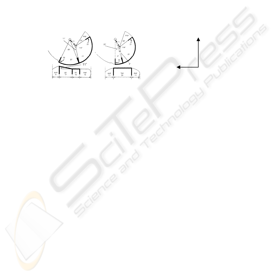
horizontal surface. Lateral tibial plateau has 3 sections; Anterior Horn Facet 11mm,
Tibial Articular Facet [TAF] 24mm, Posterior Horn Facet 11mm [7, 9] (Figure 1).
In the present work femur is assumed to be fixed and tibia moves relative to the
femur and gravity is assumed to be opposite direction in order to contact continued
between femur and tibia during flexion. The tibia is assumed to begin its motion from
rest while the knee was fully extended.
Friction forces are neglected because of the extremely low coefficient of friction of
articular surfaces [1].
In the absence of joint axial compressive loads the effect of menisectomy on joint
motion is minimal compared with that of cutting ligaments [16]. Since loading
conditions are limited to those where the knee joint is not subjected to external axial
compressive loads, the menisci thus not included in the present model [1].
y
z
M L
Fig. 1. Diagram of sagittal sections of medial [left] and lateral [right] tibio-femoral
components.
The contact force between tibia and femur is formalized as:
Fn=k [g
e
]+step[g,0,0,dmax,cmax] dg/dt
(1)
where k [46.58 N/mm] is the stiffness coefficient, g is penetration [mm], e [4] is a
force exponent, dmax [1cm] is the penetration limit cmax is the maximum damping
coefficient [97.19 N/mm/sec], dg/dt is the penetration velocity.
Patton [1993] took the penetration length as 1 cm for foot, but Blankevoort et al [5]
revealed that the articulate thickness for the knee is 2 mm, so 50% of the cartilage
thickness as penetration length is taken.
The single component force is applied to flex the knee from the center of mass of
the tibia as presented in [1] and Blankevoort et.al. [1, 5-6].
Fq = Ae
[-4.75[t/to]2
sin[πt/t
o
] (2)
where A and t
o
are the amplitude and the pulse duration, respectively. Forcing pulses
of this can be simulated experimentally. Forcing pulse duration is assumed as 140N
and 0.1 respectively.
A co-ordinate system for the normal knee based on posterior femoral circles has
been proposed by [11]. The origin is located at the center of the posterior spherical
portion of the medial femoral condyle so that the origin of the system approximately
coincides with the center of rotation of the knee as defined in [7].
43

2.2 Ligamentous Forces
The model includes 13 nonlinear spring elements which represent different
ligamentous structures and capsular tissue posterior of the knee joint. Four of them
stand for the respective anterior and posterior fiber bundles of anterior cruciate
ligament [ACL] and the posterior cruciate ligament [PCL]; another four represent the
deep, oblique, anterior and posterior fiber bundles of the medial collateral ligament
[MCL], one spring represents the lateral collateral ligament [LCL], and four elements
represent the medial, lateral, oblique fiber bundles of posterior part of the capsule
[CAP]. The local co-ordinates of the femoral and tibial insertion sites of the
ligamentous structures are specified according to the data available in the literature
[3,5,15].
Ligament assumed to be a line element extending from the femoral origin to tibial
insertion, wrapping around the bone surfaces is not taken into account.
In the present study the ligaments are determined according to the force length
relationship as [21]
(3)
where e
j is the strain in the jth element, K1j and K2j are the stiffness coefficients of the
jth spring element for the parabolic and linear regions, respectively, and L
j and Loj are
its current and slack lengths, respectively. The linear range threshold is specified as e
1
= 0.03 [1,4,13].
Values of the stiffness coefficients of the spring elements used to model the
different ligamentous structures are taken from the data available in the literature [1].
The slack length of each spring element is obtained by assuming an extension ratio e
j
at full extension and using it to evaluate the spring element’s slack length, L0j, from its
length at full extension which can be calculated from the coordinates of the attaching
points. The values of the extension ratios are specified according to the data available
in the literature [3,5]. It is verified that the selected extension ratios did not produce
nonanatomical strains [i.e., strain levels that indicate ligamentous failure] over the
whole range of motion.
3 Results
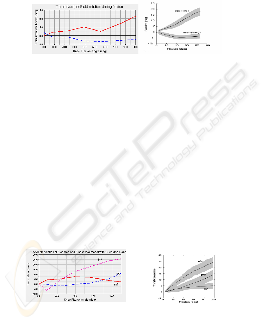
The comparison of internal and external rotation during passive knee flexion data are
shown in Figure 2. The behavior of the graphics of flat surfaces simulation and
natural rotation of tibia are different. In [7] based simulation, tibial rotation is lower
then normal during knee flexion. Tibial internal rotation is around 2 - 4° between 10 -
40° of knee flexion and rotated internally between 40 - 65°. Even though 65° knee
flexion tibial rotation is trying to catch the normal rotation, tibia has reached only 12°
internal rotation which is below the normal according to [20].
44
Int/Ex
t
a/a
Fig. 2. Comparison of int-ext rotation during knee flexion. Freeman and Pinskrova based
simulation (left), and Knee rotaion from Wilson et. al.(right).
In simulation based on Freeman and Pinskerova translations, tibial attachment of
pACL is in range except the antero-posterior translation in first 20° flexion. Tibia
translated forward during the first 20° where it is expected to translate to the
backward (Figure 3).
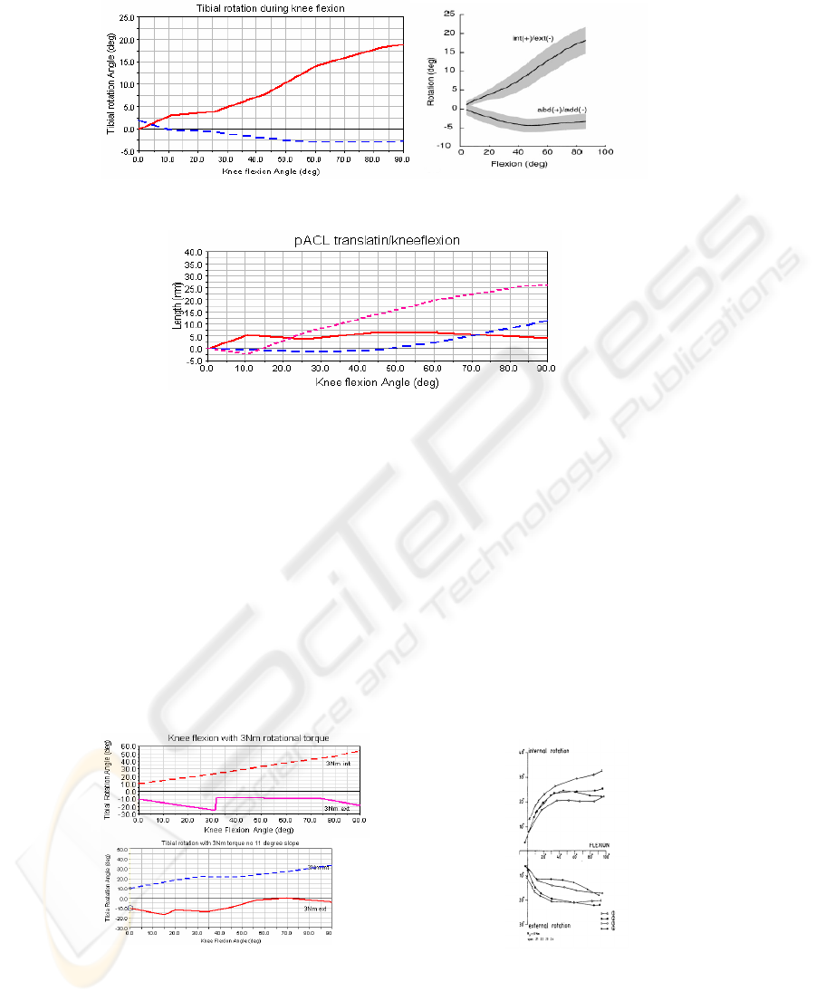
11° slope of tibial external facet is removed and the surface of the external facet and
the posterior part of the tibia provided to be on the same level. So that magnitude of
tibial internal rotation increased (Figure 4).
The internal rotation and adduction during the knee flexion is in range of normal
knee which revealed in Wilson et al 24.
The translation of tibial insertion point of pACL relative to femur during knee
flexion is in the range of normal translation described in Wilson et al’s work (Figure
5). The backward translation of pACL attachment reduced
Position of medial and lateral condyle contact point is simulated as in Pinskerova
2000. Medial femoral EF to FF rock occurred at 36°, femoral FF is in contact with
tibial FF from 36° to 90° knee flexion.
Lateral Femoral EF to FF rock occurred around 5° and from 5 to 90° femoral FF is
in contact with the tibia in slopped model. EF to FF rock is occurred at 10° flexion in
flattened tibial surface. After 10° FF contact lasts till 90° as in the literature [11]. For
the flattened medial tibial surface EF to FF rock occurred at 30° flexion and FF
contact with femoral FF till 120° flexion as revealed in Pinskerova et al work 2000
To analyze the behavior of the knee under loading conditions, 3Nm internal and
external force applied from the location of tibial center of mass as described in
Blankevoort et al [4-7]. The results for the model with and without 11° slope is
compared to the literature results (Figure 5) [5].
Fig. 3. Comparison of simulation with 11° slope (left) and Knee rotation from Wilson et.
al.(right).
45
i/e
a/a
Fig. 4. Natural internal rotation during knee flexion after 11° slope is removed.
p/a
p/d
m/l
Fig. 5. Translation of pACL during knee flexion. Freeman and Pinskrova based simulation.
Tibial internal rotation is increased linearly and reached 60° tibial rotation at 90° knee
flexion, external rotation with 3Nm external torque is in normal range for the Iwaki
and Pinskerova based simulation [9].
Even though tibial internal rotation with 3Nm torque is in normal range, tibial
external rotation is lower then normal after 35° of flexion for external rotation torque
in simulation without 11° tibial slope.
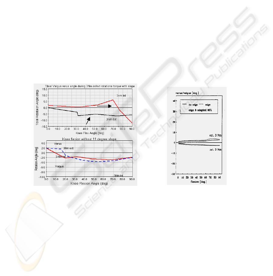
Knee varus / valgus rotation during the application of 3 Nm internal/external
rotational torque is also studied. The results are compared with Blankevort et al
(Figure 6) [6].
According to the results, valgus occurs with internal load and with external load till
75° knee flexion for 11° tibial slope. After 75° flexion valgus rotation is observed.
Valgus rotation is seen for internal and external load after 30° flexion for flattened
medial tibial surface model. Before the 30° flexion valgus rotation has occurred
(Figure 6).
With slope
Without slope
Fig. 6. Comparison of 3Nm loading torque with Blankevoort et al, Freeman and Pinskrova
based simulation (left), and Knee rotation from Blankevoort et. al.[1991](right).
46
4 Discussion
A review of the literature reveals that there is no published anatomical dynamic knee
model based on Freeman et al works [4] which describes the anatomy of the articular
surfaces and their movement in the normal tibio-femoral joint by some combination
of MRI, CT, RSA or fluoroscopy. During building anatomical dynamic knee model,
natural tibial rotation is achieved by removing 11° tibial slope. The aim of the study is
to observe the effect of 11° tibial slope to the tibio-femoral movement and to build the
most carefully sectioned tibio-femoral dynamic knee model by guidance of Freeman
et al 2005.
Tibial internal rotation during knee flexion is lower then the normal with 11° slope.
The slope on the medial tibial surface decreases the rotation by blocking tibial internal
rotation and allowing external rotation in 0 - 40° knee flexion. Between 40 - 65°, 11°
slope tackles the medial flexor facet and pushes the tibia into its external rotation.
After 65° contact moves to the posterior tibial surface and faster internal rotation is
occurred.
For the flat surface tibia demonstrated natural internal rotation. Abduction and
abduction rotation with and without 11° medial tibial slope are in the allowed limits
(Figure 2, 4).
(a) (b)
With 11
o
tibial slo
p
eslo
p
e
internal
external
Fig. 7. Comparison of internal and external 3Nm loading torque on a) valgus / varus rotation
with and without 11
o
tibial slope, b) Blankevoort et. al. (right).
Translation of most posterior location of anterior cruciate ligament is followed.
Antero-posterior translation is in normal range except first 20° part of knee flexion in
original model. In 20° knee flexion, tibia moves forward instead of backward in the
slopped model. The backward movement might be resource from hitting EF to the
slope and produce a contra force to forward motion. It may be a cause of damping
coefficient of contact formulation, which make tibia jump on femoral EF. Due to the
absence of the slope, smoother forward movement occurs in flat tibial surface.
47

Position of each part of the lateral and medial plateau relative to femur during knee
flexion is specially revealed in Pinskerova et al 2000. For the medial components;
from 0 - 10°: Femoral EF contacts with tibial EF, from 10 - 30°: EF should be rock to
FF, from 30 - 120°: Femoral FF is in contact with tibial FF. EF to FF femoral rock
occurring at 36° in simulation with slope which was late relative to the normal. EF to
FF rock at 30° knee flexion in flatten tibial model. After that, the rock contact match
with literature [9,15].
For the lateral compartment; from 0 - 10° EF, or FF in absence of EF, should be in
contact [5]. Femoral FF-to-FF rock is occurred at 5°, 10° flexion in slopped and is
flattened model respectively which are within the allowed limits. From 10 to 90° FF
is in contact with the tibia, over 90° tibia contact shared with PHF [17]. After the 10°
FF is in contact with tibial FF as literature.
To analyze loading conditions on both models, 3Nm rotational torque was applied
[5]. Higher and a linear manner tibial internal rotation is seen with internal load and
lower external rotation for external load in slopped model. Tibial internal rotation is
in range during internal load in flattened tibial model. However the external rotation
was decreased in flattened model.
The coefficients of the ligaments are obtained directly from the Abdel-Rahman and
Hefzy 1998, but the co-ordinates of the ligament attachments taken from
Crowninshield et al 1976. In Crowninshield et al 1976 medial collateral ligament is
represented as four fibers which are anterior, posterior, deep and oblique although
Abdel-Rahman and Hefzy 1998 MCL represented as three fibers, posterior fiber is
missing. In our study anterior fiber coefficients is used for posterior and anterior
fibers to compensate the absence of posterior fiber. Arcuate popliteal ligament of
posterior capsule which represented in Abdel-Rahman and Hefzy 1998 is not included
because of absence of location co-ordinates in Crowninshield et al 1976. The reason
of obtaining coordinates of ligament attachments from Crowninshield et al 1976 is the
origin co-ordinates are not defined clearly in Abdel-Rahman and Hefzy 1998.
Valgus rotation occurs by applying external rotational torque, varus by internal
rotational torque [5]. Valgus rotation and first 75° varus rotation by ±3Nm rotational
torque are in normal range for slopped model. The reason of varus rotation after 75° is
the sliding of medial tibial plateau backward and the loss of contact with flexor facet.
Valgus rotation is seen with internal rotation torque as normal although varus
rotation is only seen in 30° flexion in flattened tibial model. Valgus rotation is
observed by external rotation load after 30°. The reason of varus rotation might be
resource from excessive ligament strain or anatomical inefficiencies.
Coronal and transverse plane representation is not clear as sagittal plane in
Freeman, Pinskerova and Iwaki [7, 9, 15]. The radii of the spheres for representing
tibio-femoral articular surface are also used for coronal plane radii. The radius
differences might perform the unnatural valgus rotation by application of external
load.
The limitation of the present study is neglecting friction force because of the
extremely low coefficient of friction of the articular surface [1]. The MCL is modeled
as a straight line segment connecting the femoral and tibial attachments, while the
natural MCL wraps around the tibial plateau [20]. Meniscus and joint capsules are not
modeled because of their complex structures [2]. Some loads (around 4kg which is
weight of shank and foot) are still applied to the knee as it was flexed due to provide
48

continued contact between tibia and femur by assuming the gravity as upward
direction.
The results show that tibial internal rotation during flexion is within the normal
limits for the model without 11° anterior tibial slope. Posterior translation of tibial
attachment of pACL and sliding and rolling motion of the tibia over femur is near
normal range in flattened tibial plateau model. Both models have showed different
behaviors in loading conditions. Flattened tibial plateau model is simulated the knee
motion within the normal range for unloaded condition.
The primary feature of the three-dimensional dynamic anatomical modeling of the
knee is variation of ligament strain to achieve reasonable loading behavior for the
knee as revealed in Blankevoort et al. (1991). Modeling of the meniscus, friction,
defined in detail contact should be well studied.
Acknowledgements
This project is supported in part by TUBITAK (The Scientific and Technological
Research Council of Turkey) grant number 104S508. The project has been
coordinated at the Institute of Biomedical Engineering in Boğaziçi University. Gait
analysis experiments have been conducted at the
Motion Analysis Laboratory of
Istanbul University, School
of Medicine.
References
1. Abdel-Rahman E.M., Hefzy M.S.: Three-dimensional dynamic behavior of the human knee
joint under impact loading J. Biomech 1998,Vol 20,pp.276-90
2. Andriacchi, T.P., Mikosz R.P., :Hampton S.J. and Galante O. A statically indeterminate
model of the human knee joint, Biomechanics syposium AMD.1977.23,227-239
3. Beynnon B, Yu J, Huston D, Fleming B, Johnson R, Haugh L, Pope MH.: A sagittal plane
model of the knee and cruciate ligaments with application of a sensitivity analysis. J.
Biomech. Eng. 1996; 118:227–39.
4. Blankevoort, L., Huiskes, R., de Lange, A., 1988. The envelope of passive knee joint
motion. Journal of Biomechanics 21, 705–720.
5. Blankevoort L., Kuiper J.H., Huiskes R., Grootenboer H.J. Articular contact in a three-
dimensional model of knee. J. Biomech 1991,Vol 24,pp.1019-31
6. Crowninshield R. Pope H., Johnson R.J. An analytical model of the knee. . J. Biomech
1976,Vol 9,pp.397-405
7. Freeman M.A.R., Pinskerava V.: The movoment of the normal tibio-femoral joint.
J.Biomech 2005; 38[2]:197-208.
8. Huson A. Biomechanische probleme des kniegelenks, Orthopade1974;3:119-126
9. Iwaki H, Pinskerova V., Freeman M. Tibia-femoral mevomen 1: the shapes and relative
movoments of the femur and tibia in the unloaded cdaver knee. J Bone Joint Surg Br 2000;
82:1189-95
10. Kapandji IA.1970 The physiology of Joints, Churchill Livingstone.2.nd ed.,pp:72-134
11. McPherson,A.,Karrholm,J.,Pinskerova,V.,Sosna,A.,Martelli,S., 2004. Imaging knee motion
using MRI, RSA/CT and 3Ddigitization. Journal of Biomech 37, this issue,
doi:10.1016/j.biomech.2004.02.007
12. Menschik A. Mechanic dess Knigelenks. 1 Teil,Z. Orthop 1974;112:481-495
49

13. Moglo, K.E.,Shirazi-Adl, A., 2003. Cruciate coupling and screw home mechanism in
passive knee joint during extension-flexion J. Biomech 2005, May;38(5):1075-83
14. Patton J.L. Forward dynamic modeling of human locomotion .Master thesis 1993 pp:32
15. Pinskerova V, Iwaki H. Freeman M: The shapes and relative movements of the femur and
tibia in loaded cadaveric knee: A study using MRI as an anatomical tool. In:surgery of the
kneeInsall JN,Scott WN,eds.3.rd ed. Philadelphia: W.B Saunders Co.2000
16. Seedhom B.B., Suda Y.Axis of tibial rotation and its change with flexion angle. Clin Ort
2000;341:178-182
17. Shelburne K.B., Pandy M.C. A musculoskeletal model of the knee for evaluating ligament
forces during isometric contractions.J Biomech 1997;30:163-76
18. Smith P.N.Refshauge K.M., Scarvell J.M. Development of conceepts of knee kinemtaics
Arch Phys Med Rehabil 2003;84:18951902
19. The genesis of the LifeMOD® Biomechanics Modeler Virtual Biomechanics Brochure,
www.adams.com
20. Wilson D.R.,Feikes J.D., Zavatsky A.B., O’Connor J.J. The components of passive
movoment are coupled to flexion angle J. Biomech 2000,Vol 33,pp.465-73
21. Wismans J, Veldpaus and Jansen J:A three dimentional mathematical model of the knee
joint. J Biomech 1980;13:677-85
22. Zuppinger, Hdie aktive Flexion in unbelaseten Kniegelenk, Wiesbaden-verlag von
J.F.Bergmann, 1904
50
