
Airship Formation Control
Estela Bicho, Andr
´
e Moreira, S
´
ergio Diegues,
Manuel Carvalheira and S
´
ergio Monteiro
Departamento de Electr
´
onica Industrial da Universidade do Minho,
4800-058 Guimaraes, Portugal
Abstract. This paper addresses the problem underlying the control and coordi-
nation of multiple autonomous airships that must travel maintaining a desired ge-
ometric formation and simultaneously avoid collisions with moving or stationary
obstacles. The control architecture is based on the attractor dynamics approach to
behaviour generation. The airship physical model is presented and the mathemat-
ical background for the control architecture is explained. Simulations (with per-
turbations) with formations of two and three autonomous airships are presented
in order to validate the architecture.
1 Introduction
In this paper we address the problem underlying the control and coordination of multi-
ple autonomous airships that must drive maintaining a desired geometric formation and
simultaneously avoid collisions with obstacles(e.g. another airship, a building, etc... )
see Fig.1. The problem of formation control on land mobile robots has received much
attention from researchers working on cooperative robotics (see e.g. [1], [2], [3],
[13], [5], [6] and [7] for some interesting works). Research on UAV formation control
as also been a subject of growing research(e.g. [8], [9], [10]). In respect to airships,
some work is being done on loose formations of stratospheric airships that will serve
as telecommunications relays and airborne radar stations(e.g. Lockheed Martin High
Altitude Airship).
This project is the next step after the group work on semi-autonomous airships
control [11] [12], where we presented a control architecure based on the dynamical
systems approach to behavior generation(see c.f [18][20][19]). In [4], [13] and [14]
the control of formations of land mobile robots was adressed and studied.
Here we show how a set of decentralized and distributed basic control architectures
for line, column and ”oblique” formations can be used for teams of two airships. These
dynamic control architectures can then be easily combined to generate more complex
geometric formations for larger teams of airships. As examples we show teams of 3 air-
ships flying in line, column and V formation. We demonstrate the flexibility of our dy-
namic control architectures, presenting the ability to avoid sensed obstacles integrated
with movement in formation. Although we present examples for formations for teams
of 3 airships, more complex general configurations (larger number of airships) can be
solved by our approach.
Bicho E., Moreira A., Diegues S., Carvalheira M. and Monteiro S. (2006).
Airship Formation Control.
In Proceedings of the 2nd International Workshop on Multi-Agent Robotic Systems, pages 22-33
DOI: 10.5220/0001223900220033
Copyright
c
SciTePress

We assume that the airships have no prior knowledge of the environment and we
follow a master-referenced strategy for each airship in the team. The control architec-
ture of each airship is structured in terms of elementary behaviors (i.e. obstacle avoid-
ance and “keep formation” behavior). The individual behaviors and their integration
are modelled by non-linear dynamical systems and bifurcations are used to make de-
sign decisions around points at which a system must switch from one type of solution to
another. The advantage is that the mathematical properties associated with the concepts
(c.f. section 3) enable system integration including stability of the overall behavior of
the autonomous systems. The dynamical systems that govern the behavior of each air-
ship are tuned so that the movement of each airship in time is generated as a time series
of attractor (i.e. asymptotically stable) states. The benefit is that asymptotical stability
can be maintained and thus the systems are robust against environmental perturbations.
The rest of the paper is structered as follows; section 2 describes the background,
airship model and the system disturbances. In section 3, we explain how the forma-
tions are achieved and maintaned during flight. the basic configurations in line, column
and oblique are explained and how they can be combined in larger and more complex
formations. Section 4 reports on the simulation results on various scenarios with the
airship formations avoiding obstacles and changing formations. The last section reports
on the conclusions and some facts pertinent to the final results.
2 Aiship Model and Perturbations
The goal is to enable a team of lighter-than-air vehicles to autonomously navigate in
formation toward a target destination, avoiding obstacles and coping with environmen-
tal perturbations. We briefly discuss the organization of the team of mobile airships and
we outline the basic assumptions behind this work.
A team of N airships has one designated Lead airship labelled A
1
(the notion of
a Lead airship is in analogy with the work of Desai, Ostrowsky and Kumar[2]). This
airship navigates from an initial position to a final goal destination. Within the forma-
tion, each airship (except the Lead airship) depends on one of the others. Thus there are
many leaders and many followers but a unique Lead airship. We decompose the team
of N airships into N − 1 sub-teams of 2-airships each (Fig. 1). The control of each
sub-team follows a leader-follower decentralized motion control strategy (c.f. example
in Fig. 5).
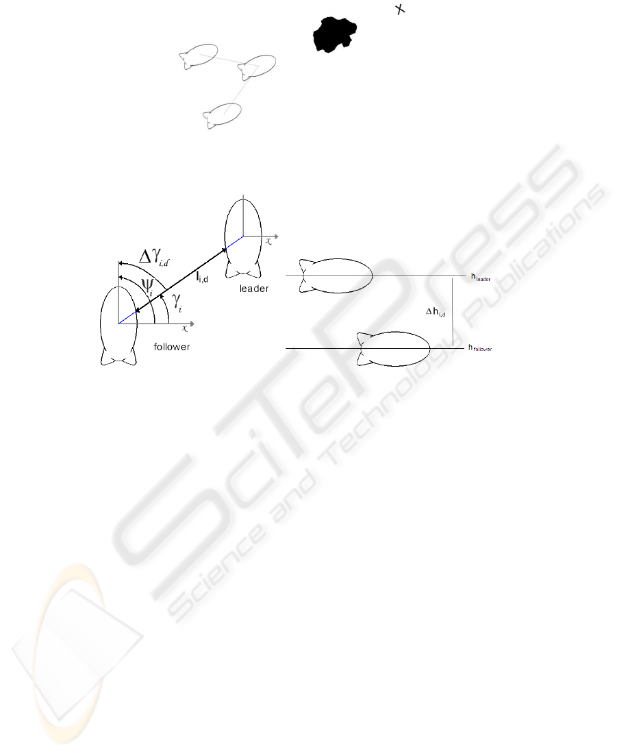
Each follower airship takes its leader as a reference point and its motion must be
controlled in order to fulfill the following task requirements (see Fig. 2): i) To maintain a
desired relative angle between the leader and the follower, ∆γ
i,d
; ii) maintain a desired
distance to the leader, l
i,d
; iii) maintain a desired altitude to the leader, ∆h
i,d
; and iv)
simultaneously avoid collisions with obstacles that may appear.
2.1 Airship Kinematics
Each airship is a balloon in which the lift is independent of flight speed, what is called
aerostatic lift. Its kinematics description is based on the reference frames presented in
figure 3.
23
A
A
A
2
3
1
Obstacle
Target
Fig.1. Example of a team with N(=3) airships in formation. A
1
is the Lead Airship, A
2
and A
3
follows A
1
in a oblique formation.
Fig.2. a) ∆γ
i,d
is the desired relative angle between the follower airship and its leader. l
i,d
is the
desired distance of the follower to the leader. γ
i
is the angle at which the follower sees the leader.
b) ∆h
i,d
is the desired altitude relative to the leader airship.
We use the following notation: The generalized coordinates for the airship are
η = (x, y, z, φ, θ, ψ)
T
∈ ℜ
6
(1)
where (x, y and z) denote the position of the centre of mass, relative to the earth-fixed
reference frame, and (φ, θ, ψ) are the three Euler angles (i.e. roll, pitch and yaw angle)
and represent the orientation of the airship (see [15], [16] or [12]). Therefore, the model
partitions naturally into translational and rotational coordinates
η
T
1
= (x, y, z)
T
∈ ℜ
3
η
T
2
= (φ, θ, ψ)
T
∈ ℜ
3
(2)
The linear and angular velocity vector with coordinates in body-fixed reference frame-
{w’} (see Fig.3) is
v = (v
x
, v
y
, v
z
, ω
x
, ω
y
, ω
z
)
T
∈ ℜ
6
(3)
which can be decomposed into:
υ
T
1
= (v
x
, v
y
, v
z
)
T
∈ ℜ
3
υ
T
2
= (ω
x
, ω
y
, ω
z
)
T
∈ ℜ
3
(4)
24
ay
obs
ay
tar
a
a
y
Target
Obstacle
y
xx
xx’
ay’
{w}
{w’}
e
obs
tar
a
e
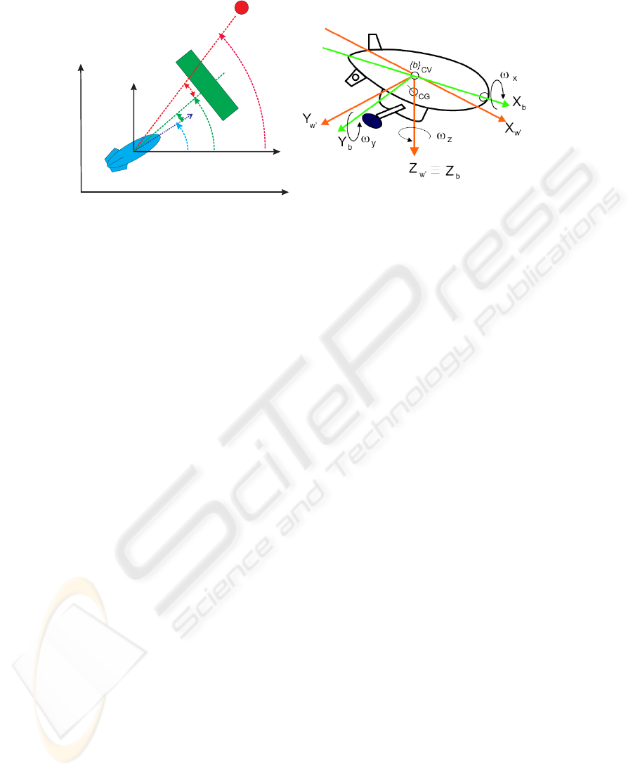
Fig.3. a) Desired task for the lead airship is movement toward the target location while avoiding
obstacles. Constraints for the yaw control (i.e. ψ) are the directions at which obstacles and target
lie as seen from the current position of the airship, i.e. ψ
obs
and ψ
tar
. Obstacle challenges the
movement toward the target location. ǫ
obs
and ǫ
tar
are given by the vision system. b) We define
three coordinate frames: i) Earth-fixed reference frame {ω}(X
ω
, Y
ω
, Z
ω
); ii) moving coordinate
frame b (X
b
,Y
b
,Z
b
) fixed to the airship and origin coincident with the centre of gravity (CG) (i.e.
body-fixed) and iii) w (X
ω
, Y
ω
, Z
ω
) is simply a translation of the earth-fixed reference frame w
to the airships centre of the gravity.
The airships flight path relative to the earth-fixed coordinate system is given by a
velocity matrix transformation:
˙η
1
= J
1
(η
2
)v
1
(5)
The body-fixed angular velocity vector υ
2
and the Euler rate vector ˙η
2
= (
˙
φ,
˙
θ,
˙
ψ)
are related through a transformation matrix according to:
˙η
2
= J
2
(η
2
)v
2
(6)
For further details on the Jacobeans J
1
(η
2
) and J
2
(η
2
) please refer to [16].
2.2 Airship Dynamics
The airship dynamics can be expressed by the following nonlinear dynamic equation of
motion:
M ˙v + C (v) v + D (v) v + g (η) = τ (7)
where variables are described in the reference frame of airship {w’} and τ is the vector
with the control inputs, i.e. forces (Fx, Fy, Fz) and torques (Nx , Ny, Nz):
τ = (τ
T
1
, τ
T
2
) (8)
τ
T
1
= [F
x
, F
y
, F
z
]
T
(9)
25
τ
T
2
= [N
x
, N
y
, N
z
]
T
(10)
The matrix M is the mass matrix (including added mass terms), C is the Coriolis
and centrifugal forces matrix, D is the aerodynamic damping matrix, g is the restoring
force (gravity and buoyancy)
In order to get a more realistic behaviour we use the non-linearized model of the
airship making the airship model time dependent. This means that C is:
C =
0 0 0 mz
G
ω
z
−m x
G
ω
y
− v
z
m x
G
ω
z
+ v
y
0 0 0 −mv
z
m z
G
ω
z
+ x
G
ω
x
mv
x
0 0 0 −m
z
G
ω
x
− v
y
−m z
G
ω
y
+ v
x
mx
G
ω
x
−mz
G
ω
z
mv
z
m
z
G
ω
x
− v
y
0 I
zz
ω
z
−I
yy
ω
y
m
x
G
ω
y
− v
z
−m z
G
ω
z
+ x
G
ω
x
m z
G
ω
y
+ v
x
−I
zz
ω
z
0 I
xx
ω
x
m
x
G
ω
z
+ v
y
−mv
x
−mx
G
ω
x
I
yy
ω
y
−I
xx
ω
x
0
(11)
It is not in the scope of this paper to go into further details on this (and also be-
cause space is limited) , but if you wish to further explore these items please check
[15][16][17]. The comprehensive non-linearized airship model is:
˙x
xy
=
−M
−1
xy
(D
xy
+ C
xy
) −M
−1
xy
g
xy
J
xy
[0]
3×3
x
xy
+
M
−1
xy
B
xy
[0]
3×2
u
xy
(12)
˙x
xz
=
−M
−1
xz
(D
xz
+ C
xz
) −M
−1
xz
g
xz
J
xz
[0]
3×3
x
xz
+
M
−1
xz
B
xz
[0]
3×2
u
xz
(13)
The general mass matrix is simplified for the xy and xz system, the same is true for the
entire matrix presented in the above systems.
The perturbed state variables for the heading direction (xy) matrix are x
xy
= (v
y
(t),
ω
x
(t), ω
z
(t), y(t), ψ(t), φ(t))
T
and the system input is u
xy
= F y; while for the xz
matrix they are x
xz
= (v
x
(t), v
z
(t), ω
x
(t), x(t), z(t), θ(t))
T
and u
xz
= (F x, F z)
T
.
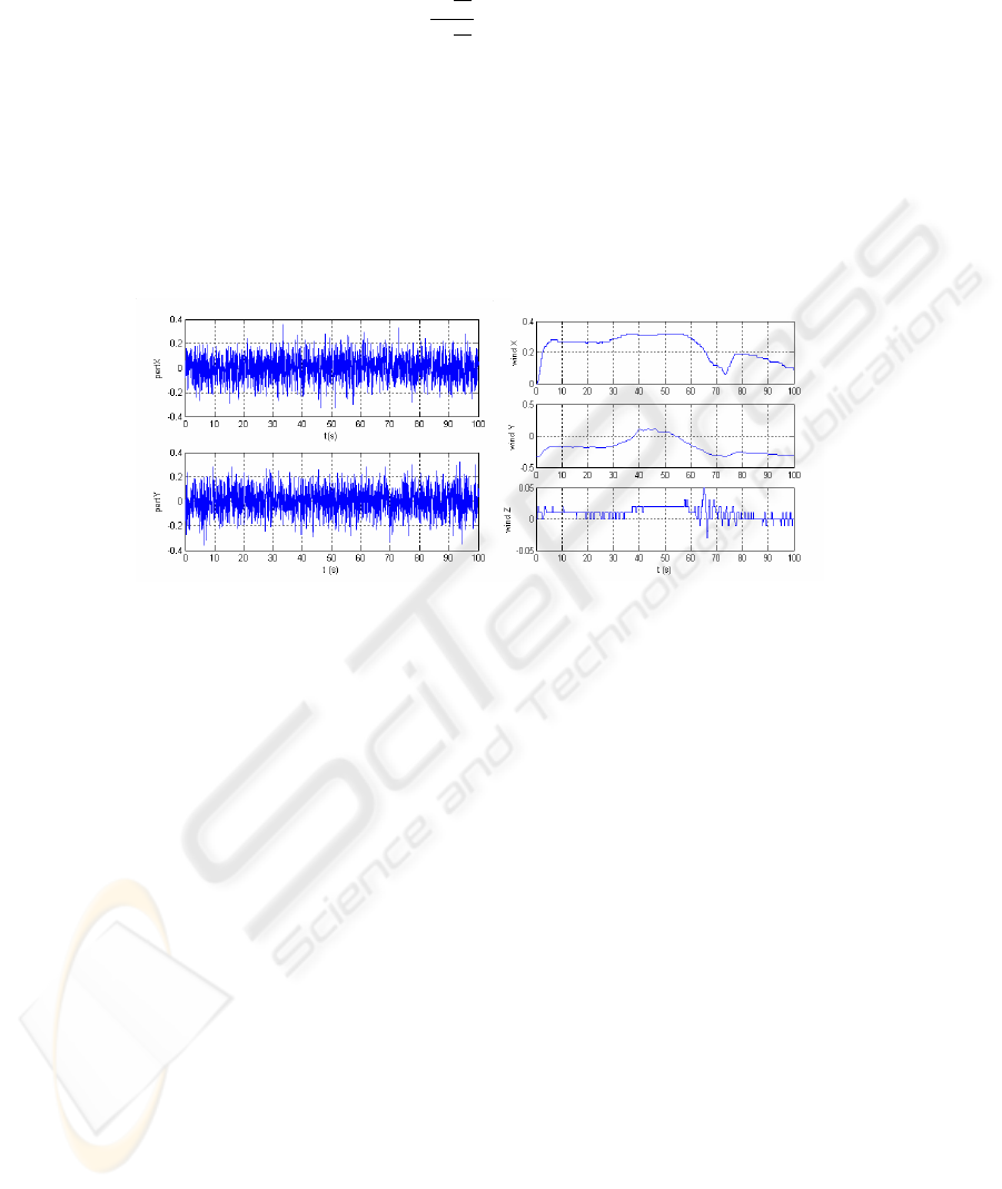
2.3 Environmental Disturbances
In order to test the robustness of the controller design we simulate the behaviour of the
airship with perturbations acting along the flight path, the perturbations are added to
the corresponding simulink models taking into account the Jacobean matrixes used (see
[12] for further details). Two types of environmental perturbations are simultaneously
considered and simulated: turbulence and wind. Both contributions were limited to a
maximum of one quarter of the airship thrusters maximum torque.
Turbulence. By definition turbulence is a state of fluid flow in which the instantaneous
velocities exhibit irregular and apparently random fluctuations so that in practice only
statistical properties can be recognized and subjected to analysis. With this in mind a
perturbation model with stochastic white noise properties was used. This perturbation
affects the airship along the longitudinal and translational axis (see Fig. 4, panel A).
Wind. The second perturbation used is a gust wind. The wind model that we used
can be found in the Matlab Simulink aerospace block set. The mathematical form is as
follows:
26
u
w
= W
6
ln
z
z
0
ln
20
z
0
, 1 ≤ z ≤ 300m (14)
where u
w
is the mean wind speed, W
6
is the measured wind speed at an altitude of
6m, z is the airship altitude, and z
0
is a constant equal to 0.0045 for Category C flight
phases and 0.18m for all other flight phases. We considered phase C (terminal flight)
due to the fact that this is the one that we feel is more adequate to a slow moving airship
(see Fig. 4, panel B). The effect of the wind on the airship frame is obtained through
the use of the corresponding Jacobean matrixes: J
1
for the heading system and J
2
for
the translation control system (see [11]).
A B
Fig.4. In panel A we can see a stochastic perturbation acting. In panel B we can see the wind.
These are the plots of the perturbations that acted on the airships during the simulation in Fig. 8.
3 Building Airship Formations
Our approach is based on the so called Dynamic Approach to Behaviour Generation
([18][19][20]). To model the airships flight behaviour we use its heading direction ψ
(i.e. yaw), forward velocity, v
x,b
, and altitude, z. Behaviour is generated by continu-
ously providing values to these variables, which control then the airships motors. The
time course of each of these variables is obtained from (fixed point) solutions of dy-
namical systems. The attractor solutions (asymptotically stable states) dominate these
solutions by design. In the present design the controller that governs the behavioural
dynamics of ψ(t), v
x,b
(t) and altitude z(t) is defined as a set of differential equations:
˙
ψ
i
= f(ψ
i
, parameters)
˙v
x,b,i
= g(v
x,b,i
, parameters) i = follower1, f ollower2, ...
˙z
i
= h(z
i
, parameters)
(15)
Task constraints define contributions to the vectors fields f , g and h. The complete
control architecture for the trajectory generation of the lead airship is described in [12]
27
in detail and we will not enter into any particular details in this paper. Next we build the
vector fields which erects an attractor at z
leader
+ ∆h
i,d
with relaxation
˙z
i
= −λ
z
(z
i
− z
leader
+ ∆h
i,d
) with λ
z
> 0 (16)
where z
leader
is the targets altitude and defines the desired valuefor the airships
altitude and λ
z
is the relaxation rate.
Now, consider two airships that navigate in a world, keeping the distance between
them constant. Then, we state that they are either in a column formation, if one is exactly
behind the other (see figure 5.a)), or in a line formation, if they navigate side-by-side
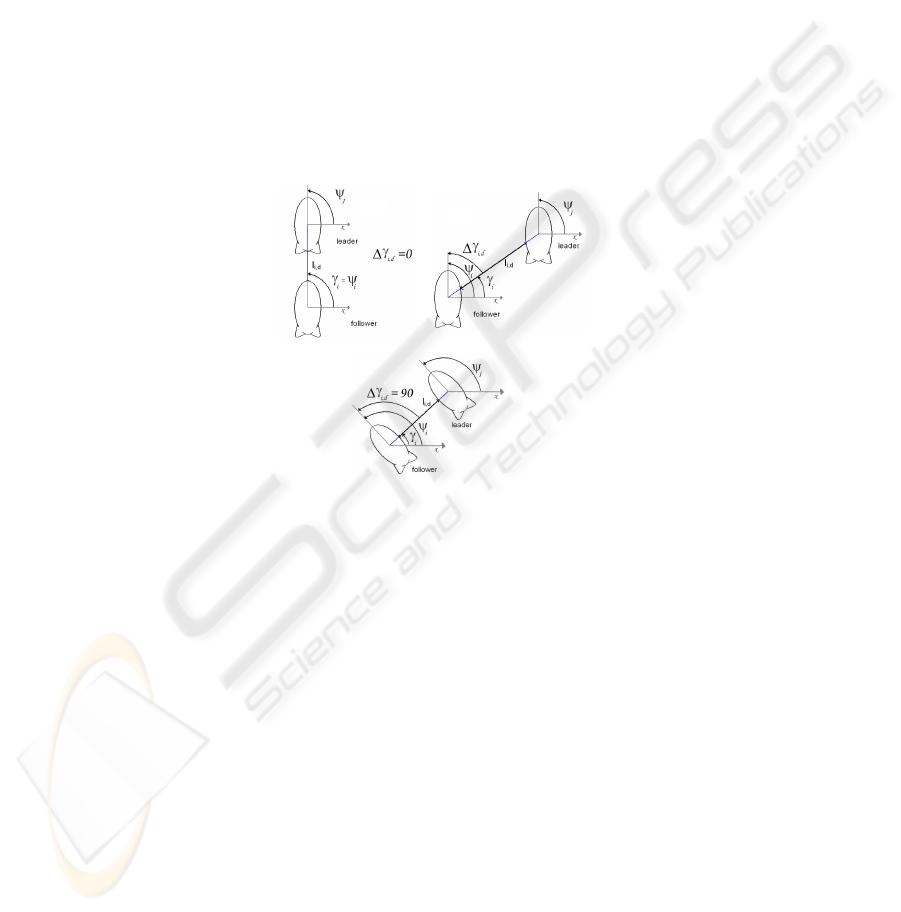
(see figure 5.c)), or in an oblique formation, otherwise (see figure 5.b)).
From this set of basic two airship formations, more complex ones can be derived,
as we will see later in section 3.4. Next, in sections 3.1 to 3.3 we present the control
architecture for each of these two airship formations.
A)
B)
C)
Fig.5. Possible formation for teams with only two airships. Note that i will refer to the leader
and j to the follower(s). The airships can either be in a) column formation; b) oblique formation;
c) line formation. The heading direction of the leader and the follower are, respectively, ψ
i
and
ψ
j
. γ
i
is the direction at which the follower sees the leader. l
i,d
is the desired distance between
both airships. ∆γ
i,d
is the desired difference between the followers heading and the direction at
which sees the leader.
3.1 Two Airships in Column
A dynamical system that causes a follower airship to navigate in column formation,
maintaining a constant distance, with its leader is:
˙
ψ
i
= f
col,i
= −λ
col
sin (ψ
i
− γ
i
) (17)
This dynamical system ensures that the airship steers to the desired heading direc-
tion, ψ
i
(the direction at which the follower sees its leader), by making it an assimptot-
28

ically stable state of the system. Parameter λ
col
(> 0) is the strength of attraction to the
attractor and corresponds to the relaxation rate.
Path velocity is controlled to ensure that the follower adequates its velocity to the
leader’s one, while trying to maintain the desired distance to it. This is accomplished
by making the value of the desired velocity equal to
v
i,d
=
v
j
− (l
i,d
− l
i
)/T
2c
if l
i
≥ l
i,d
−v
j
− (l
i,d
− l
i
)/T
2c
else
(18)
T
2
C is a parameter that smoothes the airship movement, by controlling its accelerations
and decelerations.
3.2 Two Airships in Oblique
A dynamical system that causes a follower airship to navigate in an oblique formation,
maintaining a constant distance and relative orientation, with its leader is:
˙
ψ
i
= f
oblique
(ψ
i
)
= f
attract
(ψ
i
) + f
repel
(ψ
i
) (19)
where each term defines an attractive force (k = attract, repel)
f
k
(ψ
i
) = −λ
oblique
λ
k
(l
i
)sin(ψ
i
− γ
k
) (20)
where the first contribution, f
attract
, erects an attractor at a direction
γ
attract
= γ
i
+ ∆γ
i,d
− π/4 (21)
The strength of this attractor (λ
oblique
λ
attract
(l
i
) with λ
oblique
fixed), increases with
distance, l
i
, between the two airships:
λ
attract
(l
i
) = 1/(1 + exp (−(l
i
− l
i,d
)/µ)). (22)
The second contribution, f
repel
, sets an attractor at a direction pointing away from
the leader,
γ
repel
= γ
i
+ ∆γ
i,d
+ π/4 (23)
with a strength (λ
oblique
λ
repel
(l
i
)) that decreases with distance, l
i
, between the airships,
λ
repel
(l
i
) = 1 − λ
attract
(l
i
). (24)
The attractor location of the resultant vector field, is thus dependent on the distance
between the two airships. When the distance between the two airships is larger than
the desired distance the attractive force erected at direction γ
attract
is stronger than the
attractive set at direction γ
repel
. Their superposition leads to an attractor at a direction
still pointing towards the movement direction of the leader airship. Conversely, when
the distance between the two airships is smaller than the desired distance, the reverse
holds, i.e. the attractive force set at direction γ
attract
is now stronger than the attractive
force at direction γ
repel
. The resulting oblique formation dynamics exhibits an attractor
29

at a direction pointing away from the leader’s direction of movement. When the airships
are at the desired distance the two attractive forces have the same strength which leads
to a resultant attractor at the direction γ
i,d
= γ
i
+ ∆γ
i,d
. Path velocity is controlled
exactly in the same way as for column formation.
3.3 Two Airships in Line
A dynamical system that causes a follower airship to navigate in a line formation, main-
taining a constant distance, with its leader is similar to the one of oblique formation.
The only difference lies in ∆γ
i,d
, which is fixed and equal ±π/2 depending on the
follower driving on the right or left of the leader.
In line formation, the path velocity does not depend only on the distance and ve-
locity of the leader, but we also have to take into account the heading direction of the
leader and the direction at which it is seen by the follower. A set of heuristic rules have
been written that make the follower accelerate or decelerate depending on the leader’s
pose relative to the follower:
v
i,d,line
= DE
1
· v
j
(1 − |sin(γ
i
)|) +
+ DE
2
· v
j
(1 − |cos(γ
i
)|) +
+ AC
1
· v
j
(1 + K
v
|sin(γ
i
)|) +
+ AC
2
· v
j
(1 + K
v
|cos(γ
i
)|) (25)
where DE
1
, DE
2
, AC
1
and AC
2
are mutually exclusive activation variables that em-
bed the relative attitude of the follower airship regarding the leader. They are set and
reset by testing the direction at which the leader is seen by the follower and the heading
direction of the leader (see [13] for details).
3.4 N-airship Formations
Teams of airships with more than two airships are built by specifying pairs of leader-
follower teams and stating the particular configuration to achieve. A complete team
specification is accomplished by means of a formation matrix:
S =
L
1
∆γ
1,d
l
1,d
∆h
1,d
L
2
∆γ
2,d
l
2,d
∆h
2,d
... ... ...
L
N
∆γ
N,d
l
N,d
∆h
n,d
(26)
For a team of N airships, where each airship is identified by a specific identification
number, the formation matrix has N rows and four columns. Row i relates to the airship
with identification number i. The contents of the columns specify the values that char-
acterize a formation, l
i,d
(cm) and ∆γi, d(rad) in columns two and three, respectively,
the identification number of this airships leader and the fourth column, ∆h
i,d
(cm), is
the altitude difference to the leader airship. The lead airship is identified by having its
row with l
i,d
= 0 and ∆γi, d = 0, while the third column is the distance it should stop
from the target and the fourth column is the desired altitude for the formation(see Fig. 6
for an example).
30
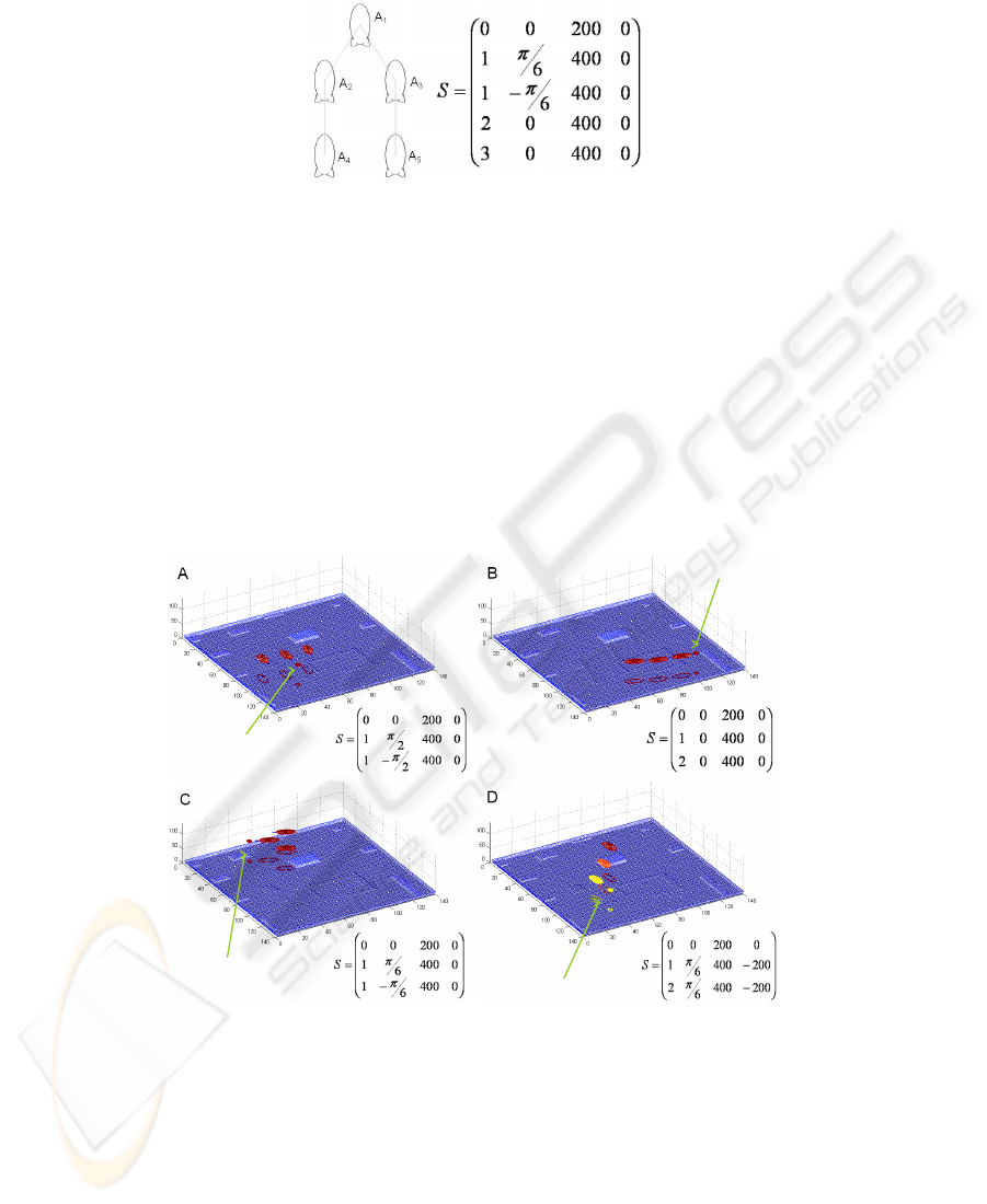
Fig.6. Example of a formation. airship A
1
is the Lead airship, airship A
2
follows A
1
on the
left side and maintaining an oblique formation, airship A
3
follows A
1
on the right side and
maintaining an oblique formation. airship A
4
follow airship A
2
in a column formation. airships
A
5
follow airship A
3
maintaining a column formation.
4 Results
In figure 7 we can see a simulation run where the possible configurations are depicted.
The airships change from line formation to column formation after reaching a waypoint.
At the next waypoint the formation changes to a V formation and at the final waypoint
they change to an oblique formation where the airships are at different altitudes
Waypoint
Waypoint
Waypoint
Waypoint
Fig.7. Simulations of the possible configuration with three airships. In panel A we can se the
airships in a line formation, in B the airships are in a column formation, in C in V formation and
in D in oblique formation with the airships at different altitudes.
In figure 8 we can observe the airships moving in a cluttered environment main-
taning formation (as close as possible) and avoiding obstacles. Depicted here is a case
31
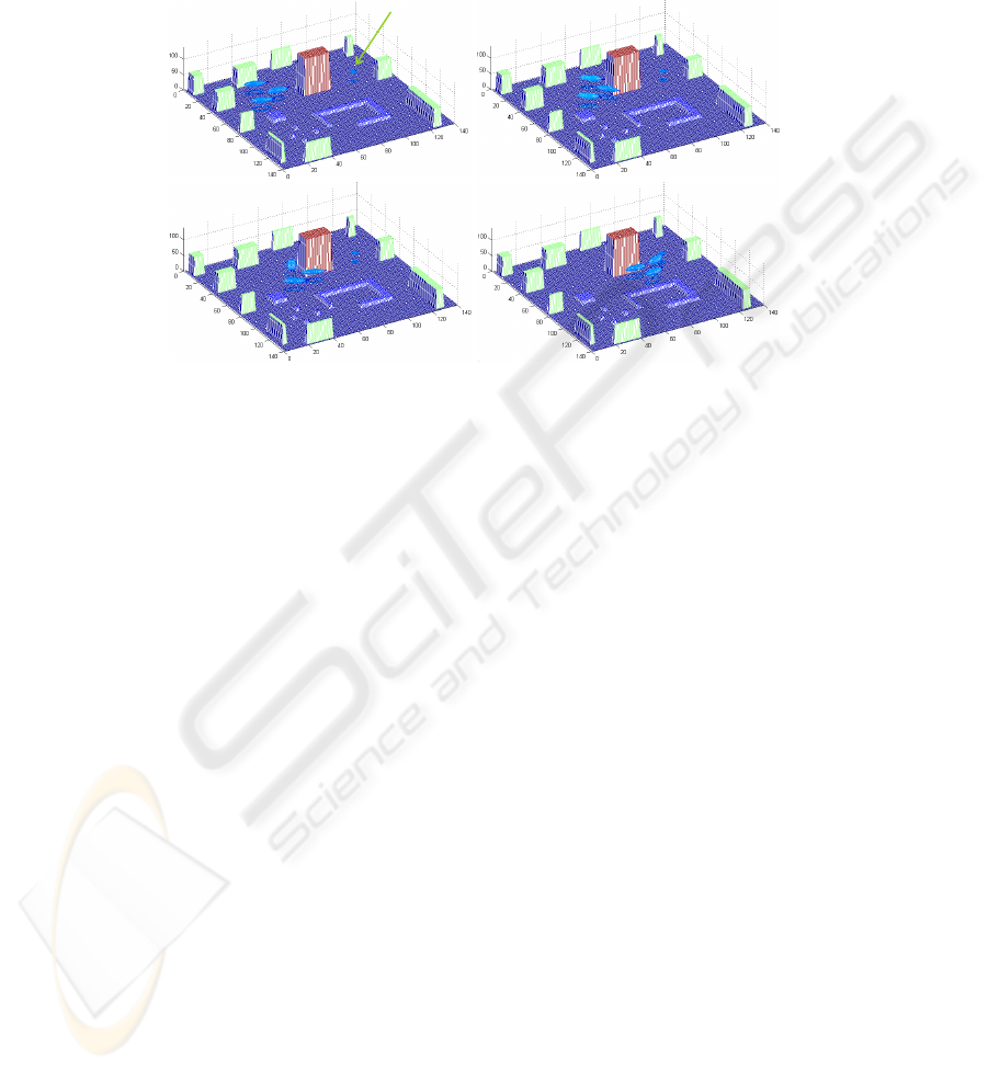
simmilar to the one that is depicted in figure 1. The target is placed behind an obstacle
and the Leader airship travels to that position. The Followers airships follow the master
in a oblique formation avoiding obstacles and keeping formation.
Target
A
B
C
D
Fig.8. In panels A through D we can see the airship formation traveling to a target position while
avoiding an obstacle in its flight path.
5 Conclusions
We demonstrated that the formation control architecture is capable of controling n-
airship formations using simple behaviours. These simple behaviours are the column,
line and oblique formations of two airships. All N-airship formations can be ”built”
from these simple behaviours. These behaviours enable the formation to avoid station-
ary obstacles.
The simulation efforts were conducted in the presence of perturbations on the main
axis of motion. Although the model of the airship is inertial, we must note that the
formation control is done at a kinematic level, where the behaviour based approach to
non-linear dynamical systems generates the next reference point for the airship control
variables. It is expected that the airship actuators are capable of ”following the orders”
given by the dynamical system. The actuator model is also taken into account during
the simulation, nevertheless, the dynamical system does not generate forces or torques
to be applied directly, it generates reference values to be followed by the robot. As with
everything this has advantages and disadvantages. The main advantage is the fact that,
with some parameters adjustmentes, the control arquitecture can be used to control any
kind of airhip - the control architecture is not model dependent. On the other hand, it
is expected that the physical platform be able to perform adequatly to the references
provided.
32

References
1. T. Balch and M. Hybinette: Social Potentials for scalable Multi-robot Formations, in IEEE
Int. Conf. Robotics and Automation, 2000
2. J. Desai, J. Ostrowski and V. Kumar: Modeling and Control of Formations of Nonholo-
nomic Mobile Robots, in IEEE Transactions on Robotics and Automation, 905-908, Decem-
ber 2001,
3. M. A. Lewis and K. Tan: High precision formation control of mobile robots using virtual
structures, in Autonomous Robots,volume 4, 387-403, 1997
4. S. Monteiro and E. Bicho: A Dynamical Systems Approach to Behavior-based Formation
Control, in IEEE Int. Conf. Robotics and Automation, 2606-2611, 2002
5. A. Paulino and H. Ara
´
ujo: Control Aspects of Maintaining Non-Holonomic Robots in Ge-
ometric Formation, in 9th International Symposium on Intelligent Robotic Systems, July
2001,18-20
6. H. Yamaguchi: A cooperative hunting behavior by mobile-robot troops, in The International
Journal of Robotics Research,931-940, September, 1999
7. P. K. C. Wang: Navigation Strategies for multiple autonomous robots moving in formation,
in Robotics and Autonomous Systems, 213-245, 1995
8. J. Sousa and T. Simsek and P. Varaiya: Task planning and execution for UAV teams, in
IEEE Conference on Decision and Control, 3804-3810, Atlantis, Paradise Island, Bahamas,
December 2004
9. R. Teo and J. S. Jang and C. J. Tomlin: Automated Multiple UAV Flight - the Stanford Drag-
onFly UAV Program, in IEEE Conference on Decision and Control,4268-4273, Atlantis,
Paradise Island, Bahamas, December 2004
10. G. Inalhan and D. Stipanovic and C.J. Tomlin: Decentralized Optimization, in IEEE Confer-
ence on Decison and Control, 1147-1155, Las Vegas, Nevada, USA, March 2002
11. E. Bicho and A. Moreira and M. Carvalheira: Control of floating robots using attractor dy-
namics, in IEEE conference on Mechatronich & Robotics,107-112, Aachen, Germany, Oc-
tober 2004
12. E. Bicho and A. Moreira and M. Carvalheira and W. Erlhagen: Autonomous Flight Trajec-
tory Generation via Attractor Dynamics, in IEEE/RSJ Int. Conf. on Intelligent Robots and
Systems, 615-621, Edmonton, Canada, August 2005,
13. E. Bicho and S. Monteiro: Formation control for multiple mobile robots: a non-linear at-
tractor dynamics approach, in IEEE/RSJ Int. Conference on Intelligent Robots and Systems,
2016-2022, Las Vegas, USA, October 2003
14. S. Monteiro and M. Vaz and E. Bicho, Attractor dynamics generates robot formations: from
theroy to implementation, in IEEE International Conference on Robotics & Automation,
2582-2587, New Orleans, USA, April 2004,
15. S.B.V. Gomes: An investigation of the flight dynamics of airships with application to the
YEZ-2A, College of Aeronautics, Cranfield University, 1990
16. Thor I. Fossen: Guidance and control of ocean vehicles, John Wiley & Sons, 1994, ISBN
0-4719-4113-1
17. Leonard Meirovich: Methods of analytical dynamics, McGraw Hill, 1970, ISBN-0-486-43-
239-4
18. Estela Bicho, Dynamic approach to behavior-based robotics: design, specification, analysis,
simulation and implementation, Shaker Verlag, 2000, ISBN 3-8265-7462-1
19. A. Steinhage, Dynamical systems for the generation of navigation behavior, Shaker Verlag,
Aachen 1999
20. G. Sch
¨
oner and M. Dose and C. Engels, Dynamics of behavior: Theory and applications for
autonomous robot architectures, Robotics and Autonomous Systems, vol. 16213-245, 1995
33
