Levy Flights in the Stochastic Dynamics of Robot
Swarm Gathering
Yechiel J. Crispin
Department of Aerospace Engineering
Embry-Riddle University
Daytona Beach, FL 32114, USA
Abstract. We consider the problem of gathering a swarm of robots which is
initially randomly dispersed over a domain in the plane. A stochastic method for
the cooperative control of a swarm of mobile robots is presented. The network of
mobile robots is modeled by a swarm performing a directed random walk. The
swarm dynamics are governed by a system of stochastic difference equations. The
motion is controlled by a robot leader, which transmits the coordinates of the
gathering point to the swarm as the network cooperative control signal. We study
the case where the control signal is corrupted by noise and find that the gathering
process is robust to noise and efficient. The swarm dynamics display anomalous
diffusion and Levy flights, where the robots move along straight lines over many
time steps, followed by short random walks in the vicinity of the gathering point.
1 Introduction
The term Levy flight was introduced by Mandelbrot and is described in his book on
fractals [6] as a sequence of jumps separated by stopovers. In plates 296 and 297 in
his book, he gives the example where each stopover is a star, a galaxy or a cluster of
stars or galaxies, thus showing that the global structure of matter distribution in the uni-
verse is composed of clusters separated by Levy flights. The clusters themselves can be
decomposed into self-similar miniclusters, resulting in a fractal structure. Since then,
other phenomena have been described as displaying Levy flights and anomalous diffu-
sion. In the present work, we show that controlled swarm robotic motion is displaying
anomalous diffusion and Levy flights.
Robots are used in many practical applications such as industrial robots in manu-
facturing, spacecraft and rover robots for space exploration and unmanned air vehicles
(UAVs) for reconnaissance, surveillance and tactical military missions. Other possible
applications include underwater missions by autonomous underwater vehicles (AUVs)
such as formation control and rendezvous, search and rescue missions and exploration
and mapping of unknown environments. In many applications, single robots are em-
ployed in the performance of a given task. It has been recognized for some time, how-
ever, that the use of collaborating multiple mobile robots can have significant advan-
tages in achieving complex tasks and missions, which otherwise might not be achiev-
able with single robots. Consequently, in recent years, there has been an interest in the
J. Crispin Y. (2006).
Levy Flights in the Stochastic Dynamics of Robot Swarm Gathering.
In Proceedings of the 2nd International Workshop on Multi-Agent Robotic Systems, pages 3-12
DOI: 10.5220/0001225200030012
Copyright
c
 SciTePress

cooperative control of networked collaborating mobile robots with distributed resources
such as sensors, computing power and communications [2, 10, 8].
Consider the problem where of a group of mobile robots has been dispersed in a
given area, and that it is required to gather the robots in the vicinity of a given point.
For example, consider the case where a group of robots has to perform a mission in
a remote area, where they have landed by parachutes. The robots are now randomly
scattered in a wide area and need to be gathered into a much smaller area in the vicinity
of a designated location before starting their mission. The specific task now is for the
robots to collectively move towards the gathering point. We consider swarms on the
order of 200 robots dispersed in a two-dimensional domain on the order of 1 km by 1
km.
It is assumed that each autonomous robot is equipped with a compass and is capable
of moving in a given azimuthal direction for a given distance. Each robot has a low level
control and navigation system that can detect its location at all times and guide it from
one point in the domain to the next at the right speed and orientation. It is also assumed
that each autonomous robot is equipped with a collision and obstacle avoidance control
system for preventing collisions with other robots and obstacles. The robots network
architecture consists of a leader robot acting as a server and communicating with the
other robots as clients.
The robot swarm cooperative control method is described in the next section. Each
robot has a microprocessor computing device on board capable of running the robot
swarm algorithm. We propose to use this paradigm algorithm as a top level discrete
event controller for the cooperative control of the swarm. Each robot sends the best so-
lution found at any given time to the leader or other central processing station through
its communication channel. The leader in turn computes the global best solution and
transmits the result as a control signal to the network. The Robot Swarm Optimization
(RSO) is a stochastic population based method that belongs to the class of biologically
inspired algorithms. It is based on the paradigm of a swarm of insects performing a col-
laborative task such as ants or bees foraging for food using chemical or some other type
of communication, see for example [1] and [3]. The swarm intelligence method was
originally developed by [4] and later described in great detail in [5]. An overview of the
method as extensively applied to various function optimization problems of increasing
difficulty has recently been presented by [7]. Here the PSO method is and adapted for
use as a top level discrete event cooperative control method for a swarm of autonomous
robots.
In the next section we develop the robot swarm algorithm with communication noise
and we explain how it can be applied to solve the swarm gathering problem. In section
3, results of simulations are described for a swarm of 200 robots, gathering in a noisy
environment. We show that the robots trajectories follow Levy flights and compute the
probability distribution for the flights lengths.
2 Cooperative Control of the Robot Swarm
In developing the robot swarm cooperative control method, we incorporate physical
effects or constraints in order to implement the search method by actual mobile robots
4

such as land vehicles, autonomous underwater vehicles or autonomous unmanned aerial
vehicles. The first effect imposes a limitation on the speed of the vehicle, or equiv-
alently, a limit on the distance ∆X
max
it can move in a given typical time step ∆t.
Another effect taken into account is imperfect and noisy communication between the
robots. At any given time, communication with one or more robots can be attenuated or
corrupted by noise. Therefore, rather than assuming that the global minimum is avail-
able to the swarm at all times as in the case of perfect communication, we introduce
noise in the control signal transmitted to all members of the swarm.
The robot swarm cooperative control algorithm without any robot speed constraints
and with perfect communication consists of minimizing a function of several variables:
minimize f(X), where X ∈ Ω ⊂ R
n
and f : Ω 7→ R
subject to the side constraints
X
min
≤ X ≤ X
max
using a directed random walk process described by the following system of stochas-
tic difference equations:
X
i
(k + 1) = X
i
(k) + ∆X
i
(k + 1) (2.1)
∆X
i
(k + 1) = w(k)X
i
(k) + c
1
r
i
1
(P
i
(k) − X
i
(k))+
c
2
r
i
2
(P
g
(k) − X
i
(k)) (2.2)
Here k is the discrete time counter, c
1
and c
2
are real constants, r
i
1
and r
i
2
are random
variables uniformly distributed between 0 and 1. The superscript index i denotes robot
number i ∈ [1, N
R
] where N
R
is the number of robots in the swarm. The location P
i
(k)
is the best solution found by robot i at time t = k and P
g
(k) is the global minimum at
time t = k. The factor w(k) can be either constant or time dependent. If it decreases
with time, the search process can usually be improved as the search approaches the
global minimum and smaller steps are needed for better resolution. For example, the
parameter w(k) can be set to decrease from an initial value of w
0
= 0.8 to a final value
of w
f
= 0.2 after N time steps:
w(k) = w
f
+ (w
0
− w
f
)(N − k)/N (2.3)
The system of equations (2.1-2.2) describes a directed random walk for each robot
i in the swarm, similar to a Brownian motion of a tracer particle in a fluid. Whereas
Brownian motion is an undirected random motion, the motion of a robot in the swarm
will have a velocity that will start as a random motion, but will eventually decay as
the particle approaches a point P
i
(k) in the domain where the function reaches a local
minimum and as the swarm as a whole approaches a point P
g
(k) of the domain where
the function reaches a global minimum, that is,
5

P
i
(k) = argmin{f(X
i
(k))}
P
g
(k) = argmin{f(P
i
(k))}, i ∈ [1, N
R
] (2.4)
The following initial conditions are needed in order to start the solution of the sys-
tem of difference equations
X
i
(0) = X
min
+ r
i
∆X
max
(2.5)
∆X
max
= (X
max
− X
min
)/N
x
(2.6)
N
x
is a typical number of grid segments along each component of the position
vector X. For example, if the domain consists of a two dimensional square domain
of 1000 m by 1000 m, then with N
x
= 50, we can use a typical distance segment of
∆X
max
= 1000 m/N
x
= 20 m. If we take a typical speed of an autonomous robot
as V
c
= 1 m/s, then the typical time will be t
c
= ∆X
max
/V
c
= 20 s. We can now
measure X in units of ∆X
max
, V in units of V
c
and ∆t in units of t
c
. The equations
will then have exactly the same form in non-dimensional variables.
Placing a limit on the magnitude of the velocity component of each robot in any
given direction for a given time step, we can impose a constraint on the magnitude of
the distance traveled in any time step as:
|∆X
i
(k + 1)| < ∆X
max
(2.7)
Under these assumptions, the equations of motion of the swarm become:
X
i
(k + 1) = X
i
(k)+
sign(∆X
i
(k + 1))(min[|∆X
i
(k + 1)|, ∆X
max
]) (2.8)
∆X
i
(k + 1) = w(k)X
i
(k) + c
1
r
i
1
(P
i
(k) − X
i
(k))+
+c
2
r
i
2
(P
g
(k) − X
i
(k)) (2.9)
subject to the side constraint
X
min
≤ X
i
(k + 1) ≤ X
max
(2.10)
The signum function term sign(∆X
i
(k + 1)) is added in order to keep the original
direction of the motion while reducing the length of the step.
6

3 Swarm Gathering in a 2-D Domain
The cooperative control method described in the previous section is applied to the prob-
lem of gathering a swarm of robots at a given point in the plane. We consider a two
dimensional domain Ω ⊂ R
2
, defined by the coordinates:
X
1
∈ [X
1min
, X
1max
] = [−500, 500]
X
2
∈ [X
2min
, X
2max
] = [−500, 500] (3.1)
which forms a square of 1000 m by 1000 m, with the origin at the center of the
square. We choose the number of grid segments as N
x
= 50, so that the maximum
distance traveled by any robot in any direction X
1
orX
2
in one time step is 20 m, which
we choose as one distance unit or 1 DU. The equivalent time unit ∆t =TU= 20 s is the
time it takes a robot to travel along 1 DU at a typical speed of 1 m/s.
∆X
1max
= ∆X
2max
=
= (X
1max
− X
1min
)/N
x
= 20m = 1DU
|V
1
|
max
= |V
2
|
max
≤ ∆X
1max
/∆t = DU/T U = 1m/s (3.2)
Initially, the swarm is randomly distributed in the domain Ω or in a subset domain
of Ω. At time k = 0, the control is started and the swarm is set in motion. Each robot
in the swarm is programmed to minimize its distance from the gathering point , by
minimizing the function:
f(X
i
1
, X
i
2
) = (X
i
1
− P
g
1
)
2
+ (X
i
2
− P
g
2
)
2
(3.3)
Here the control signal P
g
= (P
g
1
, P
g
2
) transmitted to each member of the swarm
specifies the gathering point and (X
i
1
, X
i
2
) is the location of the ith robot in the swarm,
where i ∈ [1, N
R
]. The communication signal is corrupted byadditive noise η:
P
g
= (P
g
1
+ η, P
g
2
+ η) (3.4)
η = N (0, σ) (3.5)
where N (0, σ) denotes random numbers having a normal distribution with zero
mean and standard deviation σ. Without loss of generality, we choose the gathering
point at the origin, i.e., (P
g
1
, P
g
2
) = (0, 0).
For the Gaussian noise η we chose a standard deviation σ = δ∆X
1max
with δ = 5.
As the noise level is increased, say with values of δ = 10, 20, 30,it becomes more
difficult to gather all the swarm at the origin. The other parameters appearing in the
equations of motion are c
1
= c
2
= 2 and w
0
= w
f
= 0.8. The results of a simulation
of the gathering of the 200 robots are given in Figs. 1-6. The simulation was run for
N= 80 time steps. Fig.1 shows the locations of the robots as they were spread randomly
7

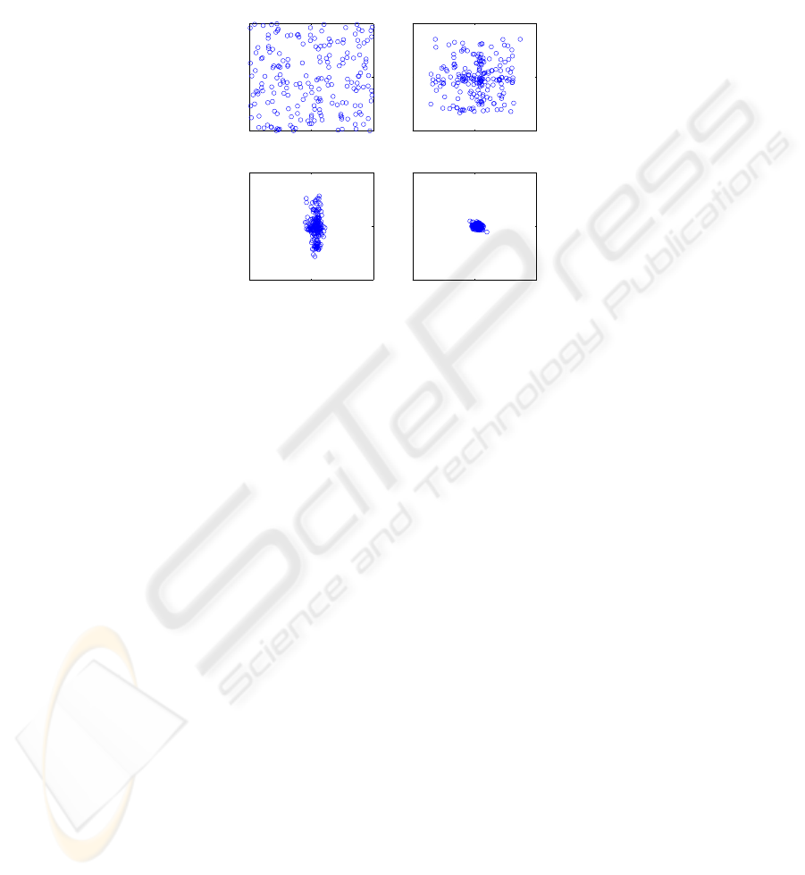
over the domain at the start of the simulation. It also shows the locations after 10 time
steps, after 15 time steps and the locations of the swarm as the robots gathered in the
vicinity of the origin after 80 time steps.
−500 0 500
−500
0
500
x1
x2
−500 0 500
−500
0
500
x1
x2
−500 0 500
−500
0
500
x1
x2
−500 0 500
−500
0
500
x1
x2
Fig.1. Swarm gathering stochastic process. Top left: Initial random swarm distribution in the
domain. Top right: After 10 time steps. Bottom left: After 15 time steps. Bottom right: After 80
time steps.
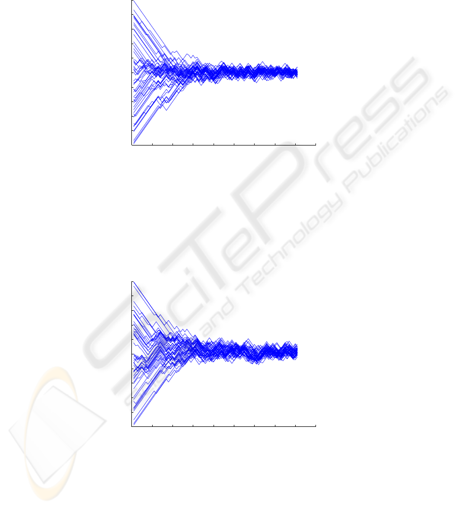
The trajectories of the first 50 robots in the swarm are shown in Figs. 2-4. Fig.2 dis-
plays the coordinates X
1
(t) as a function of time. The coordinates X
2
(t) as a function
of time are shown in Fig.3. Most Levy flights occur at the beginning of the gathering
motion, up to about 30 time steps. After that the swarm aggregates in the vicinity of the
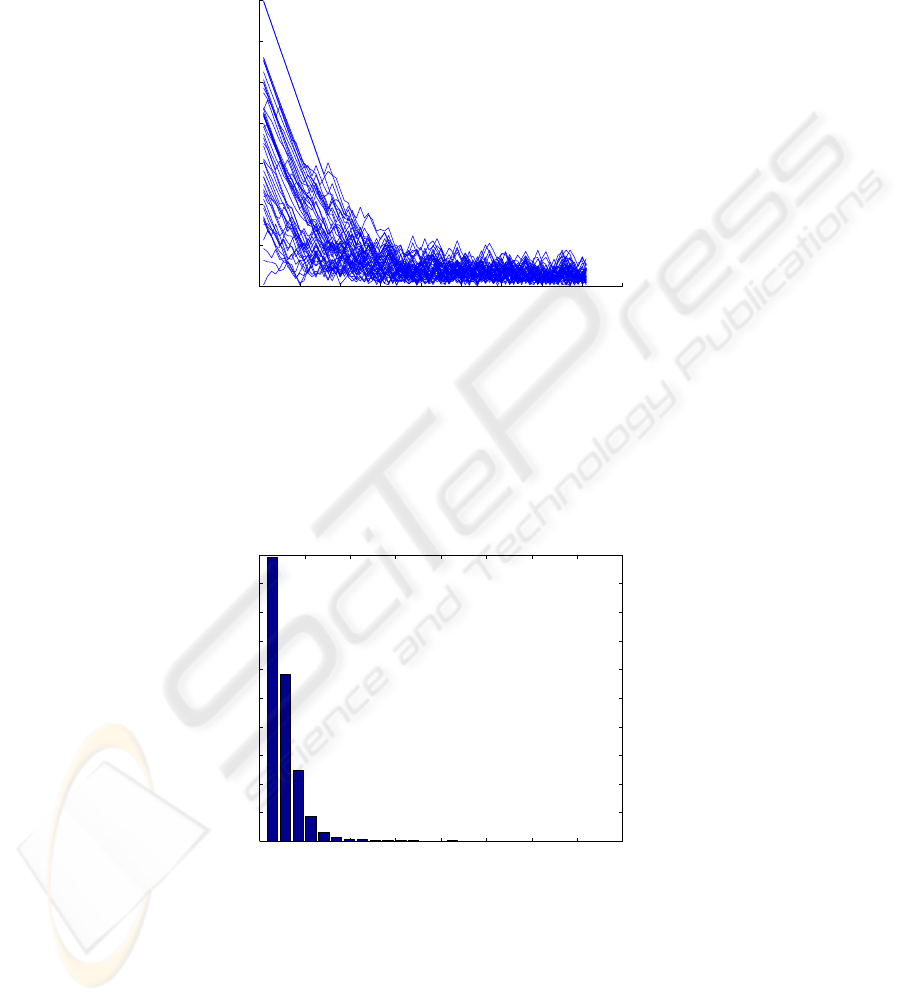
gathering point. This can also be seen in Fig.4, which displays the radial distances r(t)
from the origin, where r
2
(t) = X
2
1
(t) + X
2
2
(t) for the first 50 robots in the swarm.
In order to obtain the probability distribution of the Levy flights, the lengths of
flights along straight lines are followed for each robot in the swarm. Then the number
of flights for each given length are counted for all the robots in the swarm and put in
25 bins ordered from the shortest to the longest flights. Then a histogram is plotted
showing the frequency of occurence of the various flight lengths. Such a histogram is
shown in Fig. 5. The histogram does not follow a Gaussian distribution, but rather a
Levy distribution, which has a very long tail and an infinite variance.
Levy flights follow power laws of the form
N = (L/L
0
)
α
(3.6)
which appear as straight lines with slope α when displayed on a log-log scale
logN = αlog(L/L
0
) = αlogL − αlogL
0
(3.7)
8

0 10 20 30 40 50 60 70 80 90
−500
−400
−300
−200
−100
0
100
200
300
400
500
x1
t
Fig.2. Trajectories X
1
(t) of the first 50 robots in the swarm.
0 10 20 30 40 50 60 70 80 90
−500
−400
−300
−200
−100
0
100
200
300
400
500
x2
t
Fig.3. Trajectories X
2
(t) of the first 50 robots in the swarm.
9

0 10 20 30 40 50 60 70 80 90
0
100
200
300
400
500
600
700
r
t
Fig.4. Radial distances r(t) of the first 50 robots in the swarm.
0 50 100 150 200 250 300 350 400
0
0.05
0.1
0.15
0.2
0.25
0.3
0.35
0.4
0.45
0.5
N(L)
L(m)
Fig.5. Probability distribution of the Levy flights for the 200 robots.
10

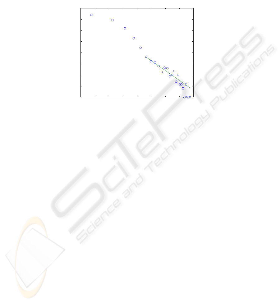
where N is the number of flights of length L and L
0
is a characteristic length. For
the noise level described above, a value of α = −2.446 and a characteristic length
L
0
= 11.62 were obtained. Such a plot is shown in Fig.6.
1 1.2 1.4 1.6 1.8 2 2.2 2.4 2.6
−4
−3.5
−3
−2.5
−2
−1.5
−1
−0.5
0
log(N(L))
log(L) (L in m)
Fig.6. Power law of the Levy flights for the tail of the distribution.
4 Conclusions
A method for the cooperative control of a group of robots based on a stochastic model
of swarm motion has been developed. The network of mobile robots is modeled by a
swarm moving randomly in the search domain with the global motion of the swarm
directed and controlled by a central unit which can be a leader robot or a central server.
The motion of each robot in the swarm is governed by a system of two stochastic dif-
ference equations. Usually, in the robot swarm method developed in this work, the best
solution found collectively by the swarm serves as the control signal for the network
of robots. However, in the swarm gathering problem, the problem is simpler, since the
coordinates of the gathering point, which serve as the control signal, are fixed, except
for additive noise that is present in the communication system. The method was used
to solve the basic problem of collaborative gathering in a two-dimensional domain. It
was found that the swarm can gather successfully in the vicinity of a designated point
in the plane despite significant noise in the network communications. Moreover, it was
found that the gathering process is efficient, in the sense that the robots trajectories ex-
hibit anomalous diffusion, performing long distance Levy flights along straight lines,
followed by local sticking random walks in a limited area of the domain in the vicinity
of the gathering point.
11

References
1. Bonabeau, E., Dorigo, M. and Theraulaz, G.: Swarm Intelligence, From Natural to Artificial
Systems. Santa Fe Institute in the Sciences of Complexity, Oxford University Press, New
York, 1999.
2. De Sousa, J.B. and Pereira, F.L.: On Coordinated Control Strategies for Networked Dynamic
Control Systems: an Application to AUVs. Proceedings of the 15th International Symposium
of Mathematical Theory of Networks and Systems, 2002.
3. Dorigo, M., Di Caro, G. and Gambardella, L.M.: Ant Algorithms for Discrete Optimization.
Artificial Life, Vol.5, pp.137-172, 1999.
4. Eberhart, R.C. and Kennedy, J.: A New Optimizer Using Particle Swarm Theory. Proceed-
ings of the 6th Symposium on Micro Machine and Human Science, IEEE Service Center,
Piscataway, NJ, 1995.
5. Kennedy, J. and Eberhart, R.C., Shi, Y.: Swarm Intelligence. Morgan Kaufman Publishers,
Academic Press, San Francisco, 2001.
6. Mandelbrot, B. B.: The Fractal Geometry of Nature. W.H. Freeman and Company, San Fran-
cisco, CA, Revised Edition, 1983.
7. Parsopoulos, K.E. and Vrahatis, M.N.: Recent Approaches to Global Optimization Problems
Through Particle Swarm Optimization. Natural Computing, Vol.1, pp.235-306, 2002.
8. Silva, J., Speranzon, A., de Sousa, J.B. and Johansson, K.H.: Hierarchical Search Strategy
for a Team of Autonomous Vehicles. IFAC 2004.
9. Solomon, T.H., Weeks, E.R. and Swinney, H.L.: Observation of Anomalous Diffusion and
Levy Flights in a Two-Dimensional Rotating Flow. Physical Review Letters, Vol.71, p.3975,
1993.
10. Speranzon, A.: On Control Under Communication Constraints in Autonomous Multi-
Robot Systems. Licentiate Thesis, KTH Signals, Sensors and Systems, Kungliga Tekniska
Hogskolan, Stockholm, Sweden, 2004.
12