
AN APPROACH TO MULTI-AGENT COOPERATIVE
SCHEDULING IN THE SUPPLY-CHAIN, WITH EXAMPLES
Joaquim Reis
Departamento de Ciências e Tecnologias de Informação, ISCTE, Avenida das Forças Armadas, 1600 Lisboa, Portugal
Keywords: Scheduling, Multi-Agent System
s, Supply-Chain Management.
Abstract: The approach to scheduling presented in this article
is applicable to multi-agent cooperative supply-chain
production-distribution scheduling problems. The approach emphasises a scheduling temporal perspective,
it is based on a set of three steps each agent must perform, in which the agents communicate through an
interaction protocol, and presupposes the sharing of some specific temporal information (among other)
about the scheduling problem, for coordination. It allows the set of agents involved to conclude if a given
scheduling problem has, or has not, any feasible solutions. In the first case, agent actions are prescribed to
re-schedule, and so repair, a first solution, if it contains constraint violations. The resulting overall agent
scheduling behaviour is cooperative. We also include some results of the application of the approach based
on simulations.
1 INTRODUCTION
In this article we present an approach to scheduling
in cooperative supply-chain production-distribution
scheduling environments, including some
unpublished details of the same work.
Scheduling is the allocation of resources over
tim
e to perform a collection of tasks, subject to
temporal and resource capacity constraints (
Baker
1974). For classical, Operations Research (OR)
based, approaches t
o scheduling see (Blazewicz
1994); for more modern approaches, Artificial
In
telligence (AI) based, see (Zweben 1994), for
i
nstance. Planning and coordination of logistics
activities (production, distribution) has been the
subject of investigation since around 1960, in the
areas of OR/Management Science (
Graves 1993).
More recently, som
e attention has been paid to
scheduling in this kind of environments (e.g., see
(
Kjenstad 1998) or (Rabelo 1998)).
In our work, the specific logistics context of
cooperat
ive supply-chain/Extended Enterprise (EE)
(
O'Neill 1996) is considered. The EE is usually
assum
ed to be a kind of Virtual Organisation, or
Virtual Enterprise, where the set of participant
agents (enterprises) is relatively stable (for concepts
and terminology see pages 3-14 in (
Camarinha-
M
atos 1999); in this last work, other approaches to
schedul
ing in this kind of context can be found).
The main features of the scheduling problem are:
a) decision is decentralised and distributed am
ong
multiple autonomous agents, b) problem solution
involves communication and cooperation among
agents, and c) scheduling can be highly dynamic.
For the modelling of the environment we adopt
th
e AI Multi-Agent Systems paradigm (
O'Hare
1996), and consider a network of agents linked
t
hrough client-supplier relationships and
communication channels. Capacity, or manager,
agents, manage, each one, the limited capacity of an
individual resource, specialised in either production
or transportation or store tasks, the last ones with
flexible durations. Producer and transporter agents
are both termed processors, as their capacity is
based on a product rate; store agent capacity is
based on a product quantity. A supervision agent
introduces work in the system, and fictitious retail
and raw-material agents define the frontiers of the
network with the outside at the downstream and
upstream extremes, respectively.
325
Reis J. (2006).
AN APPROACH TO MULTI-AGENT COOPERATIVE SCHEDULING IN THE SUPPLY-CHAIN, WITH EXAMPLES.
In Proceedings of the First International Conference on Software and Data Technologies, pages 325-332
DOI: 10.5220/0001310703250332
Copyright
c
SciTePress
b)
Request-to-Supplier
conversation model.
/
request
4
rejection
/
cancellation
/
/
cancellation
satisfaction
/
31
acceptance
/
2
5
6
r
e
-
r
e
q
u
e
s
t
/
/
r
e
-
a
c
c
e
p
t
a
n
c
e
/
r
e
-
r
e
j
e
c
t
i
o
n
/
r
e
-
r
e
q
u
e
s
t
r
e
-
a
c
c
e
p
t
a
n
c
e
/
r
e
-
r
e
j
e
c
t
i
o
n
/
transitions (message types):
receive / send
transitions (message types):
receive / send
a)
Request-from-Client
conversation model.
request
/
4
/
rejection
cancellation
/
/
cancellation
/
satisfaction
31
/
acceptance
2
6
re-re
quest
/
/
r
e
-
a
c
c
e
p
t
a
n
c
e
/
re
-
r
e
j
ec
t
i
o
n
r
e
-
r
e
j
e
c
t
i
o
n
/
5
/
r
e
-
r
e
q
u
e
s
t
r
e
-
a
c
c
e
p
t
a
n
c
e
/
c) Message types
and description.
request
- product
request, sent by a
client agent to a
supplier agent.
acceptance
- acceptance of
a previously received product
request, sent by the supplier to
the client.
rejection
- rejection of a
previously received product
request, sent by the supplier to
the client.
re-request
-
re-scheduling request,
sent by the supplier
(client) to the client
(supplier), asking to
re-schedule a
previously accepted
product request to a
given due-date.
re-acceptance
- acceptance of a
previously received re-scheduling request,
sent by the receiver to the sender of the
re-scheduling request.
re-rejection
- rejection of a
previously received re-scheduling request,
sent by the receiver to the sender of the
re-scheduling request.
cancellation
- signals giving up a
previously accepted product request, sent by
the supplier (client) to the client (supplier).
satisfaction
- signals delivery of a
previously accepted product request, sent by
supplier to client at the time of the due-date
of the product request.
Our temporal scheduling approach is described
in (
Reis 2001a) for processor agents, (Reis 2001b)]
includes a three-step procedure and processor agent
re-scheduling cases, and (
Reis 2001c) includes store
agent re-scheduling cases (our earlier work is
referred in these articles). Here we include also
some demonstration examples, taken from (
Reis
2002
), which exposes our whole model and
approach. The following sections present: the high
level agent interaction protocol used, basic concepts
underlying the approach, the steps of the approach,
some demonstration examples, and a conclusion.
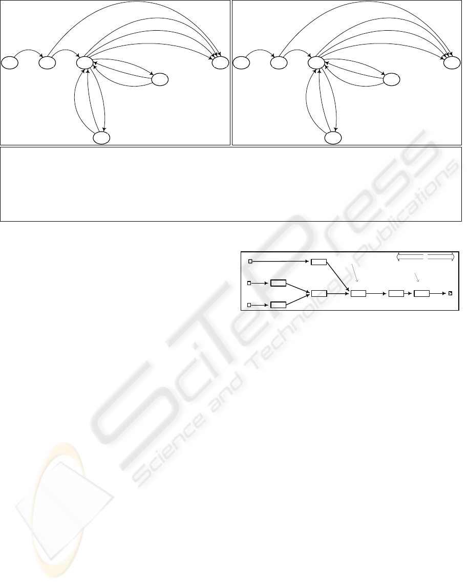
2 INTERACTION PROTOCOL
In Figure 1 we present the high level agent
interaction protocol used by capacity agents, defined
through a pair of symmetrical conversation models
(Request-from-Client and Request-to-Supplier,
shown as state diagrams) in the context of which
certain types of messages (also shown and
described) can be exchanged.
In
Figure 2 we show an example of a network
job built by agents of a hypothetical agent network
for a scheduling problem. The precedence
relationships among the tasks (the arrows forming a
tree) reflect the client-supplier relationships among
the agents.
A scheduling problem is introduced by the
network supervision agent
g
0
, through a global
interval
H=<RD,DD> (where DD and RD are the
global hard temporal limits), and a global request
from outside
d, containing retail agent
identification, product, quantity and date for
satisfaction (the request due-date,
dd=TIME(d)).
In forming the job depicted in
Figure 2, retail agent
g
14
first receives from g
0
values of DD and d, then
sends a
request type message to capacity agent
g
1
, essentially containing d. Starting from g
1
,
agents in the client-supplier tree then perform a set
of communicative actions (sending
request
messages containing local requests to one or more
suppliers to ask for task supplies). This upstream
propagation of local requests ends with the
raw-material agents
g
17
, g
18
and g
19
passing to g
0
the local requests of capacity agents
g
8
, g
11
and g
12
,
as global requests to outside. Subsequently, these
Figure 1: Conversation model state diagrams, in a) and b), and message types for the agent interaction protocol, in c).
P
O
7
i,14
network job
RT
i
,14
P
O
9
i,14
P
O
11
i,14
O
18
i,14
T
O
12
i,14
O
19
i,14
S
T
O
14
i,14
O
1
i,14
O
4
i,14
P
O
8
i,14
O
1
7
i,14
agent
g
7
task
agent
g
1
task
downstream
upstream
Figure 2: Example of a network job: job
RT
i,14
. The task
of a capacity agent
g
k
for the i
th
global request to retail
agent
g
r
is denoted by O
ir
k
,
(this task belongs to a
network job denoted by RT
i,r
); P, T and S denote
production, transportation and store tasks, respectively; the
remaining tasks are fictitious, and belong to retail and
raw-material agents (
g
14
, g
17
, and g
18
, and g
19
, which
define the limits of the agent network at the downstream
and upstream extremes).
ICSOFT 2006 - INTERNATIONAL CONFERENCE ON SOFTWARE AND DATA TECHNOLOGIES
326
agents receive from
g
0
the value of RD, and then,
acceptance messages are propagated
downstream, starting from the raw-material agents.
For each of the capacity agents, an
acceptance
message confirms its task, which is then scheduled.
According to the approach we propose (see ahead),
if any agent in the client-supplier tree detects that
the problem has no feasible solution, or receives a
rejection message from a supplier, it sends a
rejection message to its client and cancels the
accepted requests of its suppliers. This would lead to
failure in establishing the job, with rejection of the
scheduling problem by the agent network as a
whole.
After the establishment of a job for a scheduling
problem,
re-request, re-acceptance and
re-rejection messages can be used by the
agents to ask for, accept or reject re-scheduling
requests to, or from, its client or suppliers, to repair
the initial solution schedule, in the case they locally
detect temporal or capacity constraint violations. As
a last choice, agents can resort to cancellation
messages, if a feasible solution cannot be found.
This can happen because, as the environment is
dynamic, new scheduling problems appear and the
individual agent resource capacities are limited.
O
i,14
1
request
from client
request
to supplier
time
25 2827 29 30 31262420 21 22 23
d
i,14
14,1
d
i,14
1,4
h
i,14
1
H
i,14
1
FEJ
i,14
1
FJ
i,14
1
fij
i,14
1
fim
i,14
1
FEM
i,14
1
FM
i,14
1
b) Store scheduling problem.
RD
i,14
1
=22
DD
i,14
1
=31
O
i,14
7
d
i,14
7,8
d
i,14
7,9
request
from client
requests
to suppliers
fij
i,14
7
d
i,14
4,7
time
15 1817 19 20 21161410 11 12 13
FEJ
i,14
7
FJ
i,14
7
FM
i,14
7,8
fim
i,14
7,9
FEM
i,14
7,9
FM
i,14
7,9
h
i,14
7,9
h
i,14
7,8
H
i,14
7,9
H
i,14
7,8
fim
i,14
7,8
FEM
i,14
7,8
a) Processor scheduling problem.
RD
i,14
7,9
=11
RD
i,14
7,8
=10
DD
i,14
7
=21
3 COOPERATIVE APPROACH
The approach we propose is similar to some others
that operate through scheduling by repair (a first,
possibly non-feasible, solution is found which is
then repaired through search, if necessary; see
(
Minton 1992), for instance). It is based on a set of
three steps performed by each individual capacity
agent for each scheduling problem involving the
agent (specifically, involving an agent
client-supplier tree that includes the agent),
occurring after the problem is known by the agent,
i.e., after receiving the respective client
request
message. In the first two steps the approach
emphasises scheduling from a temporal perspective
and results in an overall agent cooperative
scheduling behaviour.
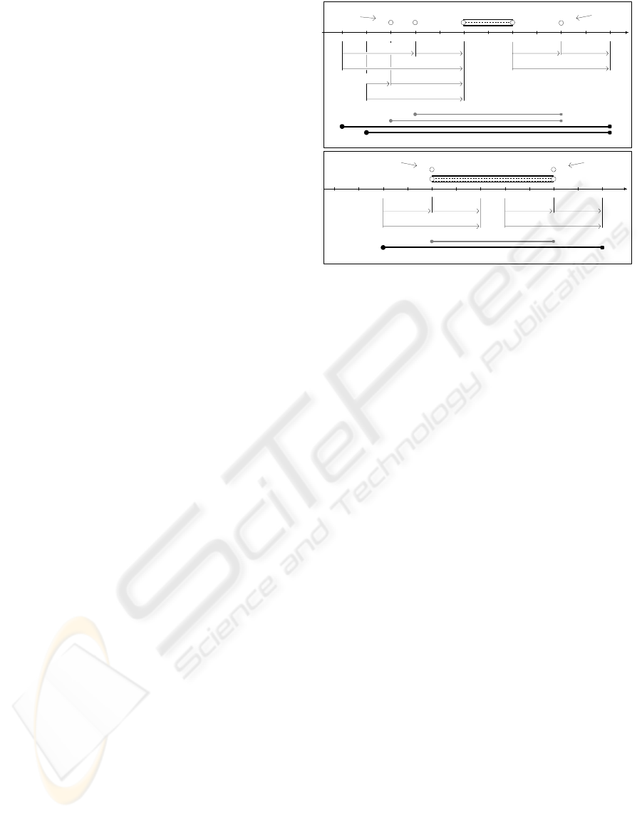
In
Figure 3 a set of temporal parameters used in
the approach are represented along timelines for a
processor agent and for a store agent; processor
g
7
and store
g
1
, involved in the job depicted in Figure
2
, are used as an example. Besides the agent task
(labelled
O) and the requests from the client and to
the supplier(s) (labelled
d), a set of temporal
intervals (labelled
h and H) and slacks (labelled FJ,
FEJ, fij, fim, FEM and FM) is shown. These are
defined in the following. In the case of
g
7
, two
suppliers are needed so, there are two
h and two H
intervals:
h
j,7
14,i
=<TIME(d
j,7
14,i
),TIME(d
7,4
14,i
)>
(j=8,9)
H
j,7
14,i
=<RD
j,7
14,i
,DD
7
14,i
> (j=8,9)
where DD
7
14,i
is the local hard temporal limit for the
end time of task
O
7
14,i
(i.e., considering all agent
tasks downstream
g
7
scheduled as late as possible),
and
RD
j,7
14,i
is the local hard temporal limit for the
start time of the
O
7
concerning to supplier
14,i
g
j
(i.e., considering all agent tasks upstream
g
7
,
starting on supplier
g
j
, scheduled as early as
possible); in determining these local temporal limits,
a minimum duration of 1 time unit for store tasks
(which have flexible duration) is considered.
For
g
7
internal downstream and upstream
slacks:
fij
7
14,i
=TIME(d
7,4
14,i
)-END(O
7
14,i
)
fim
j,7
14,i
=START(O
7
14,i
)-TIME(d
j,7
14,i
)
(j=8,9)
For g
7
external downstream and upstream
slacks:
Figure 3: Scheduling problem parameters: a) for processor
agent
g
7
, and b) for store agent g
1
(no relationship is
intended for the values in the two timelines). Symbols
with two upper indexes refer to two agents, e.g., a request
from
g
4
to g
7
in job RT
i,14
is denoted by d
i,
,
14
47
.
AN APPROACH TO MULTI AGENT COOPERATIVE SCHEDULING IN THE SUPPLY CHAIN, WITH EXAMPLES
327

FEJ
7
14,i
=DD
7
14,i
-TIME(d
7,4
14,i
)
FEM
j,7
14,i
=TIME(d
j,7
14,i
)-RD
j,7
14,i
(j=8,9)
For g
7
downstream and upstream slacks:
FJ
7
14,i
=FEJ
7
14,i
+fij
7
14,i
FM
j,7
14,i
=FEM
j,7
14,i
+fim
j,7
14,i
(j=8,9)
For g
1
intervals (stores have one h, and one H):
h
1
14,i
=<TIME(d
4,1
14,i
),TIME(d
1,14
14,i
)>
H
1
14,i
=<RD
4,1
14,i
,DD
1
14,i
>
(with a meaning for DD
1
and
14,i
RD
4,1
14,i
equivalent to
those of
g
7
). g
1
temporal slacks are defined
similarly, except for the internal slacks, which are
defined considering
INTERVAL(O
1
14,i
)=h
1
, 1
time unit minimum duration for the task and the rest
of the effective duration considered as internal slack,
being:
14,i
fij
1
14,i
+fim
1
14,i
=DURATION(O
1
)-1
14,i
Additionally, for any g
k
, we define the total
slack:
FT
k
14,i
=FJ
k
14,i
+FM
k
14,i
where
FM
k
14,i
=FM
j,k
14,i
, using for FM
j,k
14,i
the upstream
slack corresponding to the most restrictive
H
j,k
14,i
, for
processors with more than one supplier.
Assuming agents always maintain non negative
internal (
fij and fim) slacks and, in the case of
store agents, the minimum task duration is 1 time
unit, for temporal constraints to be respected, the
following conditions must hold. For processor
g
7
:
DURING(INTERVAL(O
7
14,i
),h
j,7
14,i
) ∧
DURING(h
j,7
14,i
,H
j,7
14,i
)
(j=8,9)
Similar conditions must hold for store g
1
. The
conditions mean that, for an agent scheduling
problem, an
O interval must be contained in the h
interval(s), and each
h interval must be contained in
the corresponding (same supplier)
H interval. This
is equivalent to say that all values for slacks
FJ, FM,
FEJ and FEM must be non negative. If any of the
conditions described doesn't hold, an agent must
engage in a re-scheduling activity, involving
communicative actions to agree on acceptable
temporal values of requests with the client or the
supplier(s) and, possibly, re-scheduling actions to
correct the temporal position of the task interval
(which must be, at least, inside the
H interval).
However, before engaging in such activity, an agent
must be sure that the problem is time-feasible
(otherwise it must be rejected), i.e., that the most
restrictive
H interval duration is greater than or
equal to the task duration (using for stores a
minimum of 1). This is ensured if, for any agent
g
k
:
FT
k
14,i
≥0
In order to be able to determine the values for
the end-points of
H intervals, an agent receives from
the client (via
request message) the value of the
FEJ slack; then, ensuring non negative internal
slack values for the task to be scheduled, it will send
to each supplier the supplier
FEJ value (via
request messages); the agent FEM slack values
are received from the suppliers (via
acceptance
messages), if they accept the requests; in the case the
problem is time-feasible, the agent finally schedules
its task and sends to the client the client
FEM value
(via
acceptance message). For instance, for
agent
g
7
, the H's end-points are given by
DD
7
14,i
=TIME(d
7,4
14,i
)+FEJ
7
and
14,i
RD
j,7
14,i
=
TIME(
d
j,7
14,i
)-FEM
j,7
14,i
(j=8,9); supplier g
j
FEJ
value is given by
FJ
7
14,i
+fim
j,7
14,i
, and client FEM
value by
9,8j
MIN
=
(FM
j,7
14,i
)+fij
7
14,i
; retail agent g
14
passes the value of
DD-TIME(d) to its supplier
capacity agent
g
1
, as g
1
FEJ value, and each of the
raw-material agents
g
m
(m=17,18,19) passes the
value of
TIME(d
i
km
,
,
14
)-RD to its client capacity
agent
g
k
(k=8,11,12), as g
k
FEM value.
4 STEPS OF THE APPROACH
The approach we propose is a minimal approach,
i.e., agents will only modify a scheduling problem
solution if it contains constraint violations and, in
that case, they operate minimal re-scheduling
corrections. The approach is composed of the
following sequence of three agent steps:
Step 1, Acceptance and initial solution - If any
request to a supplier was rejected, reject the request
from the client, cancel the accepted requests to
suppliers, and terminate the procedure (with failure).
Otherwise, see if the problem is temporally
over-constrained; if it is, terminate the procedure
ICSOFT 2006 - INTERNATIONAL CONFERENCE ON SOFTWARE AND DATA TECHNOLOGIES
328
(with failure) by rejecting the problem, i.e., reject
the request from the client and cancel all accepted
requests to suppliers; if it isn't, establish an initial
solution and proceed to Step 2;
Step 2, Re-schedule to find a time-feasible
solution - If the established solution is time-feasible,
proceed to Step 3. Otherwise, re-schedule requests,
or requests and task, to remove all temporal
constraint violations;
Step 3, Re-schedule to find a feasible solution -
If the solution is resource-feasible (i.e., it has no
capacity constraint violation), terminate the
procedure (with success). Otherwise, try to
re-schedule to remove all capacity constraint
violations, without violating temporal constraints; if
this is possible terminate (with success). As a last
choice, resort to cancellation, together with task
un-scheduling (terminating with failure).
time
15 17161410 11 12 136789
O
i,14
7
d
i,14
7,8
d
i,14
7,9
fim
i,14
7,9
FEM
i,14
7,9
FM
i,14
7,9
h
i,14
7,9
H
i,14
7,9
H
i,14
7,8
h
i,14
7,8
4-a) Processor case 4 situation.
time
15 17161410 11 12 136789
O
i,14
7
d
i,14
7,8
d
i,14
7,9
4-b) Situation after minimal re-scheduling.
O
i,14
7
time
15 1817161410 11 12 136789
d
i,14
7,8
d
i,14
7,9
fim
i,14
7,9
FEM
i,14
7,9
FM
i,14
7,9
h
i,14
7,9
H
i,14
7,8
h
i,14
7,8
H
i,14
7,9
2-a) Processor case 2 situation.
time
15 1817161410 11 12 136789
O
i,14
7
d
i,14
7,9
d
i,14
7,8
2-b) Situation after minimal re-scheduling.
time
15 1817 19 2016
O
i,14
7
d
i,14
4,7
1-b) Situation after minimal re-scheduling.
time
15 1817 19 2016
O
i,14
7
d
i,14
4,7
fij
i,14
7
FEJ
i,14
7
FJ
i,14
7
h
i,14
7,9
h
i,14
7,8
H
i,14
7,9
H
i,14
7,8
1-a) Processor case 1 situation.
time
1
51817 19 2016
O
i,14
7
d
i,14
4,7
3-b) Situation after minimal re-scheduling.
fij
i,14
7
O
i,14
7
d
i,14
4,7
time
1
51817 19 2016
FEJ
i,14
7
FJ
i,14
7
h
i,14
7,9
H
i,14
7,8
h
i,14
7,8
H
i,14
7,9
3-a) Processor case 3 situation.
p 1141
g8
Input
fim d fij g7 g4 g1
g11 1 2 1 fim d fij fim d fij fim d fij
fimdfij 232 121 010
131 g9 4
fim d fij g0
g12 131 H client
fim d fij 2 RD DD dd
111 01025
a) Input data.
Table 1 Step 1: Scheduling an Initial Solution p
dd = 25 1141
H = <0,10> Messages exchanged among agents
message type from to contents
request g14 g1 dd = 25 FJM / FEJ = -15
request g1 g4 dd = 24 FJM / FEJ = -15
request g4 g7 dd = 20 FJM / FEJ = -13
request g7 g8 dd = 13 FJM / FEJ = -9
request g7 g9 dd = 11 FJM / FEJ = -7
request g9 g11 dd = 6 FJM / FEJ = -5
request g9 g12 dd = 5 FJM / FEJ = -4
request g8 g17 dd = 9 FJM / FEJ = -7
request g11 g18 dd = 1 FJM / FEJ = -3
request g12 g19 dd = 2 FJM / FEJ = -2
acceptance g17 g8 FMJ / FEM = 9
acceptance g18 g11 FMJ / FEM = 1
acceptance g19 g12 FMJ / FEM = 2
rejection g11 g9
acceptance g12 g9 FMJ / FEM = 4
acceptance g8 g7 FMJ / FEM = 11
rejection g9 g7
rejection g7 g4
rejection g4 g1
rejection g1 g14
cancelation g7 g8
cancelation g8 g17
cancelation g9 g12
cancelation g11 g18
cancelation g12 g19
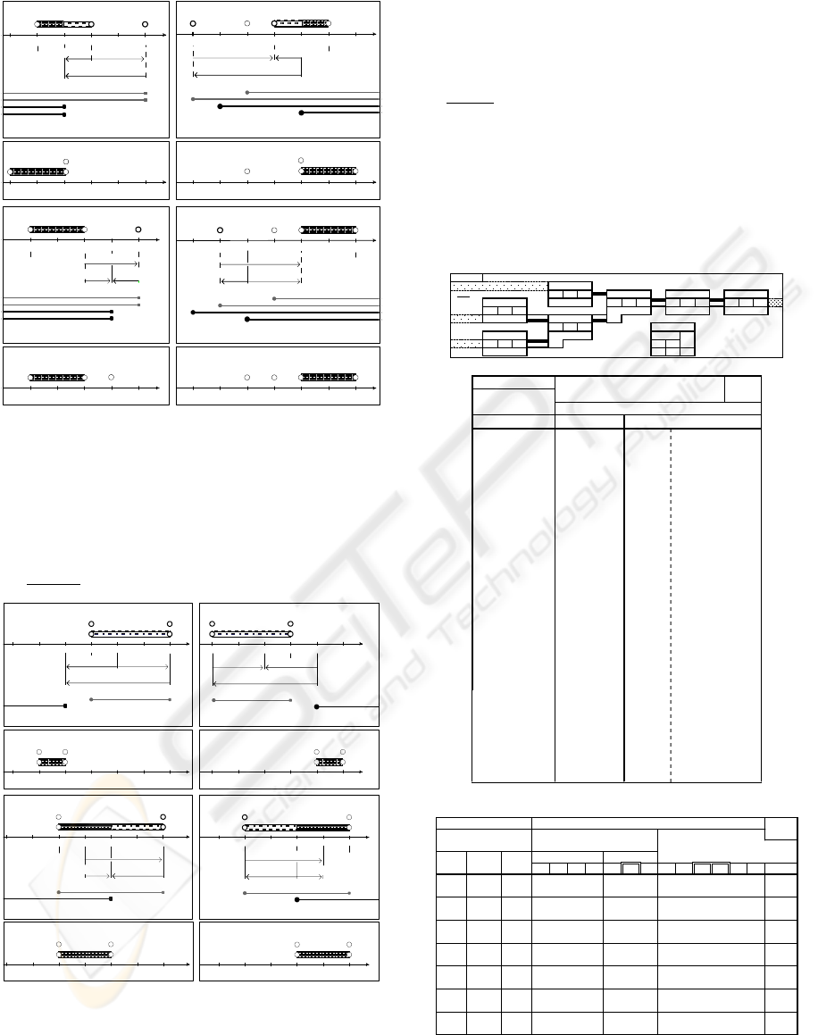
Figure 4: Examples of Step 2 re-scheduling cases 1, 2, 3
and 4, for a processor agent, with situations before, and
after, minimal re-scheduling actions.
O
i,14
1
d
i,14
1,4
time
252420 21 22 231918
d
i,14
14,1
fim
i,14
1
FEM
i,14
1
FM
i,14
1
h
i,14
1
H
i,14
1
4-a) Store case 4 situation.
time
252420 21 22 231918
O
i,14
1
d
i,14
1,4
d
i,14
14,1
4-b) Situation after minimal re-scheduling.
time
25 2827 29 30262420 21 22 231918
O
i,14
1
d
i,14
14,1
d
i,14
1,4
2-b) Situation after minimal re-scheduling.
O
i,14
1
d
i,14
14,1
time
25 2827 29 30262420 21 22 231918
d
i,14
1,4
fim
i,14
1
FEM
i,14
1
FM
i,14
1
h
i,14
1
H
i,14
1
2-a) Store case 2 situation.
O
i,14
1
d
i,14
1,4
time
2420 21 22 231918
d
i,14
14,1
FEJ
i,14
1
FJ
i,14
1
fij
i,14
1
h
i,14
1
H
i,14
1
1-a) Store case 1 situation.
time
2420 21 22 231918
O
i,14
1
d
i,14
1,4
d
i,14
14,1
1-b) Situation after minimal re-scheduling.
time
25 2827262422 23
O
i,14
1
d
i,14
14,1
d
i,14
1,4
3-b) Situation after minimal re-scheduling.
O
i,14
1
d
i,14
14,1
time
25 2827262422 23
d
i,14
1,4
FEJ
i,14
1
FJ
i,14
1
fij
i,14
1
h
i,14
1
H
i,14
1
3-a) Store case 3 situation.
b) Messages exchanged among agents during Step 1. Note the
rejection and cancellation messages.
Table 2 Step 1: Scheduling an Initial Solution p
dd = 25 Local scheduling problem 1141
H = <0,10> (for each capacity agent) Temporal slacks
capacity suppliers client dates task
agent RD rd dd DD s d e FM FEM fim fij FEJ FJ FT
g8
g17 g7 0 9 13 4 10 2 12 10 9 1 1 -9 -8 2
g11
g18 g9 01612352111-5 -4 -2
g12
g19 g9 02513143211-4 -3 0
g9
g11 g7 -- 6 11 4 7 3 10 -- -- 1 1 -7 -6 --
g12 1 5 6 4 2
g7
g8 g4 2 13 20 7 15 3 18 13 11 2 2 -13 -11 --
g9 -- 11 -- -- 4
g4
g7 g1 -- 20 24 9 21 2 23 -- -- 1 1 -15 -14 --
g1
g4 g14 -- 24 25 10 24 1 25 -- -- 0 0 -15 -15 --
Figure 5: Examples of Step 2 re-scheduling cases 1, 2, 3
and 4, for a store agent, with situations before, and after,
minimal re-scheduling actions. In order to detect cases 1
and 3, the minimum duration task interval is considered
shifted to the extreme left, and for cases 2 and 4 shifted to
the extreme right, relatively to the effective task interval.
c) Schedule data in Step 1 (incomplete, as Step 1 was terminated
with failure). Note the negative value for total slack
FT=-2,
detected by agent
g
11
.
Figure 6: Scheduling problem 1141 input and Step 1
data. Step 1, was terminated with failure, in this case.
AN APPROACH TO MULTI AGENT COOPERATIVE SCHEDULING IN THE SUPPLY CHAIN, WITH EXAMPLES
329
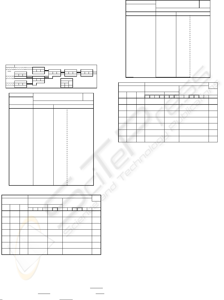
Table 3 Step 2: Re-scheduling for a p
dd = 25 Time-Feasible Solution 1155
H = <4,22> Messages exchanged among agents
message type from to contents
re-request g1 g14 dd = 22 FJ = -3
re-request g1 g4 rd = 21 FJ = -3
re-request g4 g1 dd = 21 FJ = -2
re-request g4 g7 rd = 19 FJ = -2
re-request g7 g4 dd = 19 FEJ = -1
re-request g9 g11 rd = 7 FEM = -1
re-request g11 g9 dd = 7 FM = -2
re-request g11 g18 rd = 4 FM = -2
re-request g12 g19 rd = 4 FM = -1
a) Messages exchanged among agents during Step 2.
Table 4 Step 2: Re-scheduling for a Time-Feasible Solution p
dd = 25 Local scheduling problem 1155
H = <4,22> (for each capacity agent) Temporal slacks
capacity suppliers client dates task
agent RD rd dd DD s d e FM FEM fim fij FEJ FJ FT
g8
g17 g7 4 9 13 16 10 2 12 6 5 1 1 3 4 10
g11
g18 g9 44713437001166 6
g12
g19 g9 44513415001188 8
g9
g11 g7 7711167310001156 6
g12 5 5 2 0 2
g7
g8 g4 6 13 19 19 15 3 18 9 7 1 1 0 1 6
g9 10 11 5 1 4
g4
g7 g1 13 19 21 21 19 2 21 6 6 1 1 0 0 6
g1
g4 g14 1521222221 1 22 6 6 1 1 0 0 6
b) Schedule data after Step 2.
For a time-feasible scheduling problem, this
procedure results in the agents of the client-supplier
tree building first, an initial, possibly flawed,
solution (in Step 1), which can then be repaired (in
Step 2), if necessary. Steps 1 and 2 are oriented to a
temporal perspective and concern only to a single
problem of an individual agent; Step 3 is oriented to
a resource perspective and involves all problems of
the agent at Step 3, as all the tasks of the agent
compete for its resource capacity.
p 1155
g8
Input
fim d fij g7 g4 g1
g11 1 2 1 fim d fij fim d fij fim d fij
fimdfij 232 121 010
131 g9 4
fim d fij g0
g12 131 H client
fim d fij 2 RD DD dd
111
4
In Step 2, with temporal constraint violations,
there are four possible re-scheduling cases:
case 1,
negative
FJ slack; case 2, negative FM slack(s); case
3, negative FEJ slack, and case 4, negative FEM
slack(s) (cases 1 and 2 must be tested first by the
agent, as they involve also, less critical, negative
FEJ or FEM). The cases are depicted in Figure 4 (for
processor agents) and
Figure 5 (for store agents),
together with the appropriate minimal re-scheduling
actions, using agents
g
7
and g
1
as an example.
2225
a) Input data.
Table 1 Step 1: Scheduling an Initial Solution p
dd = 25 1155
H = <4,22> Messages exchanged among agents
message type from to contents
request g14 g1 dd = 25 FJM / FEJ = -3
request g1 g4 dd = 24 FJM / FEJ = -3
request g4 g7 dd = 20 FJM / FEJ = -1
request g7 g8 dd = 13 FJM / FEJ = 3
request g7 g9 dd = 11 FJM / FEJ = 5
request g9 g11 dd = 6 FJM / FEJ = 7
request g9 g12 dd = 5 FJM / FEJ = 8
request g8 g17 dd = 9 FJM / FEJ = 5
request g11 g18 dd = 1 FJM / FEJ = 9
request g12 g19 dd = 2 FJM / FEJ = 10
acceptance g17 g8 FMJ / FEM = 5
acceptance g18 g11 FMJ / FEM = -3
acceptance g19 g12 FMJ / FEM = -2
acceptance g11 g9 FMJ / FEM = -1
acceptance g12 g9 FMJ / FEM = 0
acceptance g8 g7 FMJ / FEM = 7
acceptance g9 g7 FMJ / FEM = 1
acceptance g7 g4 FMJ / FEM = 7
acceptance g4 g1 FMJ / FEM = 9
acceptance g1 g14 FMJ / FEM = 9
5 EXAMPLES
We now present two network scheduling problem
simulation cases, together with the results of the
application of the three-step procedure described,
assuming the job depicted in
Figure 2 (see Figure 6
for the first problem, and
Figure 7, Figure 8 and
Figure 9 for the second). As input data for problem
simulation, global temporal parameters (
RD and DD
of global
H interval and date value dd=TIME(d)
of the global request from outside), as parameters
for agent
g
0
, and task durations (d) and initial
values for internal slacks (
fij and fim, which can
be further changed by agents) for each capacity
agent are given.
Figure 6 shows the initial data (a), and the
messages exchanged (b) and resulting schedule data
(c) in Step 1, for the first problem (labelled problem
b) Messages exchanged among agents during Step 1. There are
no rejection or cancellation messages.
Table 2 Step 1: Scheduling an Initial Solution p
dd = 25 Local scheduling problem 1155
H = <4,22> (for each capacity agent) Temporal slacks
capacity suppliers client dates task
agent RD rd dd DD s d e FM FEM fim fij FEJ FJ FT
g8
g17 g7 49131610212651134 10
g11
g18 g9 41613235-2 -3 1178 6
g12
g19 g9 42513314-1 -2 1189 8
g9
g11 g7 7 611167 3100-1 1 1 5 6 6
g12 5 5 2 0 2
g7
g8 g4 6 13 20 19 15 3 18 9 7 2 2 -1 1 6
g9 10 11 5 1 4
g4
g7 g1 13 20 24 21 21 2 23 8 7 1 1 -3 -2 6
g1
g4 g14 1524252224 1 25 9 9 0 0 -3 -3 6
c) Schedule data after Step 1. No agent detected a negative value
for total slack
FT.
Figure 7: Scheduling problem 1155 input and Step 1 data.
Step 1, was terminated with success, in this case.
Figure 8: Scheduling problem 1155 Step 2 data. Some
requests were re-scheduled to remove temporal
constraint violations (the negative slacks in
Figure 7-c).
ICSOFT 2006 - INTERNATIONAL CONFERENCE ON SOFTWARE AND DATA TECHNOLOGIES
330
H
interval
h
intervals
timelines
H
intervals
h
intervals
task interval
for agent
g
0
(whole network) for a capacity agent
legends fo
r
schedule intervals
network schedule 1
24 25
2524
15 2 2
21 23
2420
13 2 1
15 18
2011
6 19
10 12
913
4 16
710
116
115
25
61
413
34
52
413
2013
716
25
921
4 22
1910
5 16
0
1
2
3
4
5
6
7
8
9
10
11
12
13
-5 -4 -3 -2 -1 0 1 2 3 4 5 6 7 8 9 10 11 12 13 14 15 16 17 18 19 20 21 22 23 24 25 26 27 28 29 30
time
agent
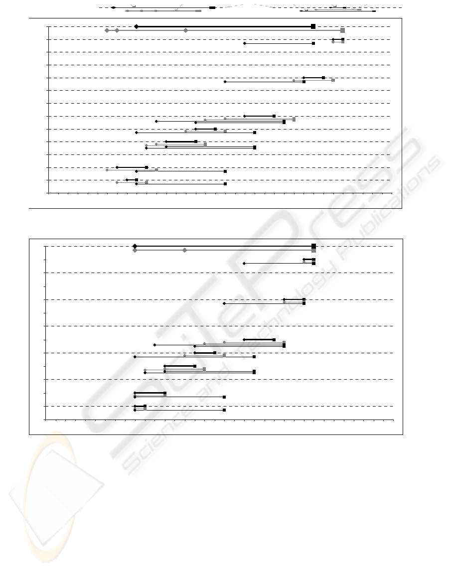
a) Schedule resulting from Step 1 (built from data in Figure 7-c). Concerning to temporal constraint violation situations experienced by the
agents, as shown, agents
g
1
and g
4
have a case 1 situation, agent g
7
has a case 3 situation, agent g
9
has a case 4 situation and agents g
11
and
g
12
have a case 2 situation.
network schedule 2
2221
21 22
2215
2119
19 2 1
2113
1815
13 19
1911
1210
139
164
107
711
511
74
47
134
54
45
134
6 19
167
449
22
224
10 19
165
0
1
2
3
4
5
6
7
8
9
10
11
12
13
- 5 - 4 - 3 - 2 - 1 0 1 2 3 4 5 6 7 8 9 10 11 12 13 14 15 16 17 18 19 2 0 2 1 2 2 2 3 2 4 2 5 2 6 2 7 2 8 2 9 3 0
b) Schedule resulting from Step 2 (built from data in Figure 8-b). All temporal constraint violations were removed.
P 1141). The problem was rejected in Step 1 (with
the initiative taken first by capacity agent
g
11
), as it
is temporally over-constrained.
Figure 7 shows the initial data (a), and the
messages exchanged (b) and resulting schedule data
(c) in Step 1, for the second problem (labelled
problem P 1155). As
Figure 7-c shows, no capacity
agent detected a negative value for total slack
FT, so
the problem is not temporally over-constrained.
As a result, no rejection or cancellation messages
are exchanged until the end of Step 1, see
Figure
7
-b. The resulting network schedule in Step 1 is
shown in
Figure 9-a. In Step 2, temporal constraint
violation situations of case 1 for agents
g
1
and g
4
, of
case 3 for agent
g
7
, of case 4 for agent g
9
, and of
case 2 for agents
g
11
and g
12
are detected. Solution
repair is accomplished by agents through inter-agent
local request re-scheduling (for all those agents),
and additional agent task re-scheduling (only for
agents
g
1
, g
4
, g
11
and g
12
), according to the
minimal actions prescribed.
Figure 8 shows the
messages exchanged (a) and resulting schedule data
(b), and
Figure 9-b shows the resulting schedule in
Step 2, for this problem. As shown by
Figure 9-b, all
temporal constraint violations found in the initial
solution (
Figure 9-a) disappeared.
Figure 9: Schedules for problem P 1155: a) after Step 1 (terminated with success), and b) after Step 2.
AN APPROACH TO MULTI AGENT COOPERATIVE SCHEDULING IN THE SUPPLY CHAIN, WITH EXAMPLES
331

6 CONCLUSION
We described an approach to multi-agent scheduling
in a cooperative supply-chain environment. The
approach presupposes the use of an agent interaction
protocol (also described), is based on a three-step
procedure prescribed for each agent involved in a
scheduling problem, and results in an individual
cooperative scheduling behaviour. In Step 1 agents
detect if the problem is temporally over-constrained
and, if it isn't, they schedule an initial, possibly non
time-feasible, solution (otherwise, they reject the
problem). The exchange of specific temporal slack
values, besides product, quantity and due-date
information, used as a scheduling coordination
mechanism, allows the agents to locally perceive the
hard global temporal constraints of the problem, and
rule out non time-feasible solutions in the
subsequent steps. Each of these pieces of
information exchanged in Step 1 corresponds, for a
particular agent, to a sum of slacks downstream and
upstream the agent in the agent network, and cannot
be considered private information of any agent in
particular. If necessary, in Step 2, agents repair the
initial solution, through re-scheduling, in order to
obtain a time-feasible one. In Step 3 any capacity
constraint violation must be removed, either through
re-scheduling, or by giving up the problem.
No specific details were given for Step 3. In fact,
this is the matter of our current and future work.
Step 3 can be refined to accommodate additional
coordination mechanisms for implementing certain
solution search strategies. For instance, strategies
based on capacity/resource constrainedness (see
[
Sycara 1991] or [Sadeh 1994]), to lead the agents on a
fast convergence to both time and capacity-feasible
solutions, including solutions satisfying some
scheduling preferences, or optimising some criteria,
either from an individual agent perspective, or from
the global perspective of the overall system.
REFERENCES
Baker 1974. Baker, K.R., Introduction to Sequencing and
Scheduling, Wiley, New York, 1974.
Blazewicz 1994. Blazewicz, J.; Ecker, K.H. ;Schmidt, G.;
Weglarz, J., Scheduling in Computer and
Manufacturing Systems, Springer Verlag, 1994.
Camarinha-Matos 1999. Camarinha-Matos, L.M.;
Afsarmanesh, H. (eds.), Infrastructures for Virtual
Enterprises, Networking Industrial Enterprises,
Kluwer Academic Publishers, Dordrecht, The
Netherlands, 1999.
Graves 1993. Graves, S.C.; Kan, A.H.G. Rinnooy; Zipkin,
P.H., (eds.), Logistics of Production and Inventory,
Handbooks in Operations Research and Management
Science, Volume 4, North-Holland, Amsterdam, 1993.
Kjenstad 1998. Kjenstad, Dag, Coordinated Supply Chain
Scheduling, PhD. Thesis, Norwegian University of
Science and Technology, 1998, Trondheim, Norway.
Minton 1992. Minton, Steven, et al, Minimizing Conflicts:
a Heuristic Repair Method for Constraint Satisfaction
and Scheduling Problems, Artificial Intelligence 58,
1992, 161-205.
O'Hare 1996. O'Hare, G.M.P.; Jennings, N.R.,
Foundations of Distributed Artificial Intelligence,
John Wiley & Sons, Inc., 1996, New York, USA.
O'Neill 1996. O'Neill, H.; Sackett, P., The Extended
Enterprise Reference Framework, in Balanced
Automation Systems II, Camarinha-Matos, L.M. and
Afsarmanesh, H. (Eds.), 1996, Chapman & Hall,
London, UK, 401-412.
Rabelo 1998. Rabelo, R.J.; Camarinha-Matos, L.M.;
Afsarmanesh, H., Multiagent Perspectives to Agile
Scheduling, Basys'98 Int. Conf. on Balanced
Automation Systems, Prague, Czech Republic, 1998.
Reis 2001a. Reis, J.; Mamede, N.; O’Neill, H., Locally
Perceiving Hard Global Constraints in Multi-Agent
Scheduling, Journal of Intelligent Manufacturing,
Vol.12, No.2, April 2001, 227-240.
Reis 2001b. Reis, J.; Mamede, N., Multi-Agent Dynamic
Scheduling and Re-Scheduling with Global Temporal
Constraints, Proceedings of the ICEIS’2001, Setúbal,
Portugal, 2001, Miranda, P., Sharp, B., Pakstas, A.,
and Filipe, J. (eds.), Vol. I, 315-321.
Reis 2001c. Reis, J.; Mamede, N., Scheduling, Re-
Scheduling and Communication in the Multi-Agent
Extended Enterprise Environment, accepted for the
MASTA'01 Workshop, EPIA'01 Conference,
December, 17-20, 2001, Porto, Portugal.
Reis 2002. Reis, J., Um Modelo de Escalonamento
Multi-Agente na Empresa Estendida, PhD thesis (in
portuguese), ISCTE 2002, Lisbon, Portugal.
Sadeh 1994. Sadeh, N., Micro-Oportunistic Scheduling:
The Micro-Boss Factory Scheduler, in Intelligent
Scheduling, Morgan Kaufman, 1994, Chapter 4.
Sycara 1991. Sycara, Katia P.; Roth, Steven F.; Sadeh,
Norman; Fox, Mark S., Resource Allocation in
Distributed Factory Scheduling, IEEE Expert,
February, 1991, 29-40.
Zweben 1994. Zweben, Monte; Fox, Mark S., Intelligent
Scheduling, Morgan Kaufmann Publishers, Inc., San
Francisco, California, 1994.
ICSOFT 2006 - INTERNATIONAL CONFERENCE ON SOFTWARE AND DATA TECHNOLOGIES
332
