
A PATTERN SELECTION ALGORITHM IN KERNEL PCA
APPLICATIONS
Ruixin Yang, John Tan, Menas Kafatos
Center for Earth Observing and Space Research (CEOSR)
College of Science
George Mason University
Fairfax, VA 22030, U.S.A.
Keywords:
Data mining, knowledge acquisition, large-scale, dimension reduction.
Abstract:
Principal Component Analysis (PCA) has been extensively used in different fields including earth science
for spatial pattern identification. However, the intrinsic linear feature associated with standard PCA prevents
scientists from detecting nonlinear structures. Kernel-based principal component analysis (KPCA), a recently
emerging technique, provides a new approach for exploring and identifying nonlinear patterns in scientific
data. In this paper, we recast KPCA in the commonly used PCA notation for earth science communities and
demonstrate how to apply the KPCA technique into the analysis of earth science data sets. In such applica-
tions, a large number of principal components should be retained for studying the spatial patterns, while the
variance cannot be quantitatively transferred from the feature space back into the input space. Therefore, we
propose a KPCA pattern selection algorithm based on correlations with a given geophysical phenomenon. We
demonstrate the algorithm with two widely used data sets in geophysical communities, namely the Normalized
Difference Vegetation Index (NDVI) and the Southern Oscillation Index (SOI). The results indicate the new
KPCA algorithm can reveal more significant details in spatial patterns than standard PCA.
1 INTRODUCTION
Principal Component Analysis (PCA) has been ex-
tensively used in different fields since introduced by
Pearson in 1902 (as cited in (Von Storch and Zwiers,
1999)). This data decomposition procedure is known
by various names in different disciplines such as
Karhunen-Lo
`
eve Transformation (KLT) in digital sig-
nal processing (Haddad and Parsons, 1991), Proper
Orthogonal Decomposition (POD) in studies of tur-
bulence coherent structure with nonlinear dynamical
systems (Holmes et al., 1996), and Empirical Orthog-
onal Function (EOF) for one variable data (Lorenz,
1959) or Singular Value Decomposition (SVD) for
multiple variables (Wallace et al., 1992) applied to
earth science, in particular for climate studies.
In principle, PCA is a linear procedure to transform
data for various purposes including dimension re-
duction (factor analysis), separation of variables, co-
herent structure identification, data compression (ap-
proximation), feature extraction, etc. Consequently,
PCA results can be viewed and explained from vari-
ous perspectives. One way to interpret the PCA re-
sults is to consider the PCA procedure projecting the
original high dimensional data into a new coordinate
system. In the new system, the space spanned by the
first few principal axes captures most of the infor-
mation (variances) of the original data (Krzanowski,
1988). Another point of view, commonly used in
earth science, is to consider the PCA results of spatio-
temporal data as a decomposition between the spatial
components and temporal components. Once again,
the approximation defined by the first few principal
components gives the smallest total mean-square er-
ror compared to any other expansions with the same
number of items (Emery and Thomson, 2001).
In earth science applications, the spatial compo-
nents from the PCA decomposition are recognized
as representative patterns because the spatial com-
ponents are orthogonal to each other. Correspond-
ingly, the uncorrelated time series (temporal compo-
nents) are often used to study the relationships be-
tween the corresponding spatial patterns and a pre-
determined phenomenon such as the well-known El
Ni
˜
no, characterized by abnormally warm sea surface
temperature (SST) over the eastern Pacific Ocean.
Through this procedure, patterns can be associated
with natural phenomena. One example of such asso-
ciation is found between Normalized Difference Veg-
etation Index (NDVI) patterns and ENSO (El Ni
˜
no
195
Yang R., Tan J. and Kafatos M. (2006).
A PATTERN SELECTION ALGORITHM IN KERNEL PCA APPLICATIONS.
In Proceedings of the First International Conference on Software and Data Technologies, pages 195-202
DOI: 10.5220/0001320801950202
Copyright
c
SciTePress

Southern Oscillation) by directly using spatial com-
ponents of PCA (Li and Kafatos, 2000). Another
well-known spatial pattern is obtained by regressing
the leading principal time series from the sea-level-
pressure (SLP) to the surface air temperature (SAT)
field (Thompson and Wallace, 2000).
Although PCA is broadly used in many disciplines
as well as in earth science data analysis, the intrin-
sic linear feature prevents this method from iden-
tifying nonlinear structures. This may be neces-
sary as many geophysical phenomena are intrinsi-
cally nonlinear. As a consequence, many efforts
have been made to extend PCA to grasp nonlinear
relationships in data sets such as the principal curve
theory (Hastie and Stuetzle, 1989) and the neutral
network-based PCA (Kramer, 1991; Monahan, 2001),
which is limited to low dimensional data or needs
standard PCA for preprocessing. More recently, as
the kernel method has been receiving growing atten-
tion in various communities, another nonlinear PCA
implementation as a kernel eigenvalue problem has
emerged (Sch
¨
olkopf et al., 1998).
The kernel-based principal component analysis
(KPCA) actually is implemented via a standard PCA
in feature space, which is related to the original in-
put space by a nonlinear implicit mapping (Sch
¨
olkopf
et al., 1998). KPCA has been recently applied to earth
science data to explore nonlinear low dimensional
structures (Tan, 2005; Tan et al., 2006). Ideally, the
intrinsic nonlinear low dimensional structures in the
data can be uncovered by using just a few nonlinear
principal components. However, the dimension num-
bers of the feature space are usually much larger than
the dimension numbers of the input space. Moreover,
the variance cannot be quantitatively transferred from
the feature space back into the input space. Conse-
quently, the numbers of principal components which
contribute meaningful amounts of variances are much
larger than we commonly encounter in standard PCA
results. Therefore, we need a mechanism to select
nonlinear principal patterns and to construct the rep-
resentative patterns. In this paper, we present the
KPCA algorithms in language used in climate studies
and propose a new KPCA pattern selection algorithm
based on correlation with a natural phenomenon for
KPCA applications to earth science data.
To the best of our knowledge, this work is the first
and only effort on using KPCA in climate studies for
knowledge acquisition. Therefore, in the following
section, we first describe the PCA algorithm and then
the KPCA algorithm in language comparable to the
standard PCA applications in climate studies. Next,
we present the newly proposed KPCA pattern selec-
tion algorithm. Then we briefly discuss the earth sci-
ence data used for this work in Section 3 and describe
the results in Section 4. In Section 5, we first dis-
cuss in-depth our understanding of the KPCA con-
cepts, and finally present conclusions.
The contribution of this work includes two main
points: 1) The emerging KPCA technique is de-
scribed in the notation of PCA applications com-
monly used in earth science communities, and this
work is the first KPCA application to earth science
data; 2) A new spatial pattern selection algorithm
based on correlation scores is developed here to over-
come the problems of KPCA applications in earth sci-
ence data sets, the overwhelming numbers of com-
ponents and the lack of quantitative variance descrip-
tion.
2 ALGORITHM
KPCA emerged only recently from the well-known
kernel theory, parallel to other kernel-based algo-
rithms such as support vector machine (SVM) classi-
fication (Sch
¨
olkopf et al., 1999a). In order to compare
the similarities and the differences between standard
PCA and KPCA, in this section, we first describe the
commonly used standard PCA algorithms applied to
earth science data analysis and then the KPCA algo-
rithm for the same applications. Then, we discuss the
limitation and new issues of KPCA such as pattern
selection. Finally, we describe the new KPCA pattern
selection algorithm.
2.1 PCA Algorithm
We follow the notations and procedures common to
earth science communities to describe the standard
PCA algorithm and a variant of its implementation by
dual matrix (Emery and Thomson, 2001).
Suppose that we have a spatio-temporal data set,
ψ(~x
m
, t), where ~x
m
represents the given geolocation
with 1 ≤ m ≤ M, and t, the time, which is actually
discretized at t
n
(1 ≤ n ≤ N). The purpose of the
PCA as a data decomposition procedure is to separate
the data into spatial parts φ(~x
m
) and temporal parts
a(t) such that
ψ(~x
m
, t) =
M
X
i=1
a
i
(t)φ
i
(~x
m
). (1)
In other words, the original spatio-temporal data sets
with N time snaps of spatial field values of dimen-
sion M can be represented by M number of spatial
patterns. The contribution of those patterns to the
original data is weighted by the corresponding tempo-
ral function a(t). To uniquely determine the solution
satisfying Equation (1), we place the spatial orthogo-
nality condition on φ(~x
m
) and the uncorrelated time
variability condition on a(t).
ICSOFT 2006 - INTERNATIONAL CONFERENCE ON SOFTWARE AND DATA TECHNOLOGIES
196

The above conditions result in an eigenvalue prob-
lem of covariance matrix C with λ being the eigen-
values and φ the corresponding eigenvectors. We can
construct a data matrix D with
D =
ψ
1
(t
1
) ψ
1
(t
2
) ... ψ
1
(t
N
)
ψ
2
(t
1
) ψ
2
(t
2
) ... ψ
2
(t
N
)
... ... ... ...
ψ
M
(t
1
) ψ
M
(t
2
) ... ψ
M
(t
N
)
, (2)
where ψ
m
(t
n
) ≡ ψ(~x
m
, t
n
). Each row of matrix D
is corresponding to one time series of the given phys-
ical values at a given location, and each column is a
point in an M-dimensional space spanned by all lo-
cations, corresponding to a temporal snap. With the
data matrix, the covariance matrix can be written as
C = fac ∗ DD
′
(3)
where the apostrophe symbol denotes the transpose
operation. In the equation above, fac = 1/N.
Since the size of matrix D is M ×N , the size of ma-
trix C is M ×M. Each eigenvector of C with M com-
ponents represents a spatial pattern, that is, φ(~x
m
).
The corresponding time series (N values as a vector,
~a) associated with a spatial pattern represented by
−→
φ
j
can be obtained by the projection of the data matrix
onto the spatial pattern in the form of
−→
a
j
′
=
−→
φ
j
′
D.
The advantage of the notations and procedures
above, as normally defined in the earth science com-
munities, is that they shed light on interpretation of
the PCA results. Based on the matrix theory, the
trace of covariance matrix C is equal to the sum of
all eigenvalues. That is, trace(C) ≡
P
M
i=1
c
ii
=
P
M
i=1
λ
i
. From Equation (2) and Equation (3), we
have
c
ii
=
1
N
N
X
n=1
[ψ
i
(t
n
)]
2
, (4)
which is the the variance of the data at location ~x
i
if
we consider that the original data are centered against
the temporal average (anomaly data). Therefore, the
trace of C is the total variance of the data, and the
anomaly data are decomposed into spatial patterns
with corresponding time series for the contribution
weights. The eigenvalues measure the contribution
to the total variance by the corresponding principal
components.
Computationally, solving an eigenvalue problem of
an M × M matrix of DD
′
form is not always opti-
mal. When N < M, the eigenvalue problem of ma-
trix DD
′
can be easily converted into an eigenvalue
problem of a dual matrix, D
′
D, of size N × N be-
cause the ranks and eigenvalues of DD
′
and D
′
D are
the same (Von Storch and Zwiers, 1999). Actually,
the rank of the covariance matrix, r
C
, is equal to or
smaller than min(M, N). The summation in Equa-
tion (1) and other corresponding equations should be
from 1 to r
C
instead of M.
The element of the dual matrix of the covariance
matrix:
S = fac ∗ D
′
D (5)
is not simply the covariance between two time series.
Instead,
s
ij
=
1
N
M
X
m=1
[ψ
m
(t
i
)ψ
m
(t
j
)] , (6)
can be considered as an inner product between two
vectors which are denoted by columns in the data ma-
trix D and are of M components. One should note
that spatial averaging does make sense in earth sci-
ence applications for one variable, unlike in tradi-
tional factor analysis. Nevertheless, the data values
are centered against the temporal averages at each lo-
cation. Due to this fact, the dual matrix S cannot be
called a covariance matrix in strict meanings.
Since the matrix S is of size N × N, the eigen-
vectors are not corresponding to the spatial patterns.
Actually, they are corresponding to the temporal prin-
cipal components, or the time series, a(t). To obtain
the corresponding spatial patterns, we need to project
the original data (matrix D) onto the principal time
series by
−→
φ
j
= D
−→
a
j
(7)
with an eigenvalue dependent scaling.
2.2 KPCA Algorithms
In simple words, KPCA is the implementation of lin-
ear PCA in feature space (Sch
¨
olkopf et al., 1998).
With the same notation as we used in the previous
section for the spatio-temporal data, we can recast the
KPCA concept and algorithm as follows.
As in the case with dual matrix, we consider each
snap of spatial field with M points as a vector of M
components. Then, the original data can be consid-
ered as N M-dimensional vectors or N points in an
M-dimensional space. Suppose that there is a map
transforming a point from the input space (the space
for original data) into a feature space, then we have
Φ : R
M
→ F;
~
ψ 7→
~
X. (8)
Assume the dimension of the feature space is M
F
,
one vector in the input space,
−→
ψ
k
, is transformed into
−→
X
k
≡
−−−−→
Φ(
−→
ψ
k
) =
Φ
1
(
−→
ψ
k
), Φ
2
(
−→
ψ
k
), ..., Φ
M
F
(
−→
ψ
k
)
.
(9)
Similar to the data matrix in input space, we can de-
note the data matrix in the feature space as
D
Φ
=
Φ
1
(
−→
ψ
1
) Φ
1
(
−→
ψ
2
) ... Φ
1
(
−→
ψ
N
)
Φ
2
(
−→
ψ
1
) Φ
2
(
−→
ψ
2
) ... Φ
2
(
−→
ψ
N
)
... ... ... ...
Φ
M
F
(
−→
ψ
1
) Φ
M
F
(
−→
ψ
2
) ... Φ
M
F
(
−→
ψ
N
)
.
(10)
A PATTERN SELECTION ALGORITHM IN KERNEL PCA APPLICATIONS
197

Unlike the standard PCA case, where we can ac-
tually solve an eigenvalue problem for either DD
′
or
D
′
D depending on the spatial dimension size and the
number of observations (temporal size), we can only
define
K = fac ∗ D
Φ
′
D
Φ
(11)
for the eigenvalue problem in the feature space. This
limitation comes from the so called “kernel trick”
used for evaluating the elements of matrix K.
Comparing to the definition of s
ij
for the standard
PCA case, we will have the element of matrix K as
k
ij
= fac∗
D
Φ
′
D
Φ
ij
=
1
N
(
−−−→
Φ(
−→
ψ
i
)•
−−−→
Φ(
−→
ψ
j
)). (12)
The key of the kernel theory is that we do not need
to explicitly compute the inner product. Instead, we
define a kernel function for this product such that
k(~x, ~y) =
−−→
Φ(~x) •
−−→
Φ(~y)
. (13)
Through the “kernel trick,” we do not need to know
either the mapping function Φ or the dimension size
of the feature space, M
F
, in all computations.
The main computation step in the KPCA is to solve
the eigenvalue problem with K~α = λ~α. The eigen-
values still can be used to estimate the variance but
only in the feature space. The eigenvector, as the case
with dual matrix S in the standard PCA case, is play-
ing a role of a time series. For the spatial patterns in
the feature space, another projection, similar to that
described in Equation (7),
~v =
M
X
m=1
α
i
−−−→
Φ(
−→
ψ
i
). (14)
is needed. In practice, we do not need to compute~v ei-
ther. What we are more interested in is the spatial pat-
terns we can obtain from the KPCA process. There-
fore, we need to map back the structures represented
by ~v in the feature space into the input space. Since
the mapping from the input space to the feature space
is nonlinear and implicit, it is not expected that the re-
verse mapping is simple or even unique. Fortunately,
a preimage (data in the input space) reconstruction al-
gorithm based on certain optimal condition has been
developed already (Mika et al., 1999). In this process,
all needed computations related to the mapping can be
performed via the kernel function, and the algorithm
is used in this work.
2.3 KPCA Pattern Selection
Algorithm
Kernel functions are the key part in KPCA applica-
tions. There are many functions that can be used
as kernel as long as certain conditions are satis-
fied (Sch
¨
olkopf et al., 1998). Examples of kernel
functions include polynomial kernels and Gaussian
kernels (Sch
¨
olkopf et al., 1999b). When the kernel
function is nonlinear as we intend to choose, the di-
mension in the feature space is usually much higher
than the dimension in the input space (Sch
¨
olkopf
et al., 1998). In special situations, the number of
the dimensions could be infinite as in the case pre-
sented by the Gaussian kernel (Mika et al., 1999). The
higher dimension in feature space is the desired fea-
ture for machine learning applications such as classifi-
cation because data are more separated in the feature
space and special characters are more easily identi-
fied. However, for spatial pattern extraction in earth
science applications, the higher dimensionality in-
troduces new challenges because we cannot simply
pick one or a few spatial patterns associated with the
largest eigenvalues.
Moreover, in standard PCA, the principal direc-
tions represented by the spatial patterns can be con-
sidered as the results of rotation of the original coordi-
nate system. Therefore, the total variance of the cen-
tered data is conserved under the coordinate system
rotation. As a result, significant spatial patterns are
selected based on the contribution of variance by the
corresponding patterns to the total variance. This can
simply be calculated by the eigenvalues as discussed
in Section 2.1. In the KPCA results, the mapping be-
tween the input space and the feature space is non-
linear. Therefore, the variance is not conserved from
input space into the feature space. Consequently, al-
though the eigenvalues still can be used to estimate
the variance contribution in feature space, the vari-
ance distribution in the feature space cannot be quan-
titatively transferred back into variance distribution in
the input space.
The introduction of higher dimensions in KPCA,
that is, a large number of principal components and
the difficulty to quantitatively describe the variance
contribution in the input space by each component re-
quire a new mechanism for identifying the significant
spatial patterns. A new pattern selection algorithm is
developed (Tan, 2005) to overcome these problems as
described below.
In standard PCA applications for earth science data
analysis, the temporal components are usually corre-
lated with a time series representing a given natural
phenomenon. And the corresponding spatial pattern
is claimed to be related to the phenomenon if the cor-
relation coefficient is significantly different from zero.
In KPCA, we cannot easily identify such spatial pat-
terns, but we generally have more temporal compo-
nents, as discussed in Section 2.2. The eigenvectors
~α, i.e., the KPCA temporal components, can be used
to select KPCA components which can enhance the
correlation to the given phenomenon.
After we perform the KPCA process on a partic-
ular set of data, we utilize an algorithm to obtain a
ICSOFT 2006 - INTERNATIONAL CONFERENCE ON SOFTWARE AND DATA TECHNOLOGIES
198

reduced set of temporal components in the pattern
selection procedure. Although the variance in fea-
ture space does not represent the variance in the input
space, we can still use the eigenvalues as a qualitative
measurement to filter KPCA components which may
contribute to the spatial patterns in the input space.
We are interested in the significant KPCA compo-
nents which are associated with, say, 99.9% variance
in feature space as measured by the corresponding
eigenvalues, and treat other components associated
with very small eigenvalues as components coming
from various noises. The algorithm sorts the tempo-
ral components in descending order according to their
correlation score with a given phenomenon. Then lin-
ear combinations of them are tested from the high-
est score to the lowest, only the combinations that in-
crease the correlation with the signal of interest are
retained. The steps for combining the temporal com-
ponents are:
• The correlation score of a vector V with the signal
of interest is denoted as corr(V).
• Sort the normalized PC’s according to the correla-
tion score → PC
1
, P C
2
, . . . , P C
p
.
• Save the current vector with the highest correlation
score → V := P C
1
.
• Save the current high correlation score as cc →
cc := corr(P C
1
).
• Maintain a list of the combination of sorted PC’s
→ List{ } .
Where List.Add{1} results in List{1},
List.Add{2} results in List{1, 2} , etc...
Loop over the possible combinations of PC’s that
can increase the correlation score. If the score is
increased, then keep the combination of PC’s. The
pseudo-code for the new pattern selection algorithm
is given in Figure 1. In the pseuso-code and in the list
above, p is the number of KPCA components we are
interested in after de-noise.
V := P C
1
cc := corr(P C
1
)
List.Add(1)
FOR i := 2 TO p
IF corr(V + P C
i
) > cc THEN
V := V + P C
i
cc := corr(V + P C
i
)
List.Add(i)
END IF
END FOR
Figure 1: Pseudo-code of the pattern selection procedure.
The spatial patterns in input space are computed
based on the preimage algorithm with all selected
components (Mika et al., 1999).
3 DATA
A gridded global monthly Normalized Difference
Vegetation Index (NDVI) data set was chosen to im-
plement the KPCA. NDVI is possibly the most widely
used data product from earth observing satellites. The
NDVI value is essentially a measure of the vegeta-
tion greenness (Cracknell, 1997). As vegetation gains
chlorophyll and becomes greener, the NDVI value in-
creases. On the other hand, as vegetation loses chloro-
phyll, the value decreases.
The NDVI data used here were obtained from the
NASA data web site (GES DISC (NASA Goddard
Earth Sciences (GES) Data and Information Services
Center (DISC)), 2006). The data are of 1
0
× 1
0
latitude-longitude spatial resolution with global cov-
erage, and monthly temporal resolution with tempo-
ral coverage from January 1982 to December 2001.
Since PCA analysis usually needs data without gaps,
only data points with valid NDVI data in the whole
period are chosen in the analysis. Therefore, we
worked on global NDVI data for the 1982-1992 pe-
riod only. Before using the data with PCA or KPCA,
the NDVI data are deseasonalized by subtracting the
climatological values from the original data. For that
reason, the analysis is actually on NDVI anomalies.
In implementations, each point (location) in the
physical coordinate system (the globe in latitude-
longitude coordinates) is treated as one dimension,
and time another dimension. Consequently, the data
sets are represented in matrix format, and each col-
umn represents one month and each row element in
the column represents a grid point value. In other
words, all the latitude-by-longitude grid points for
each month will be unrolled into one column of the
data matrix. Therefore, the rows in each column rep-
resent a spatial location in latitude and longitude and
each column represents a point in time as shown in
the data matrix of Equation (2).
As a relationship between NDVI PCA patterns and
El Ni
˜
no Southern Oscillation (ENSO) was found (Li
and Kafatos, 2000), we pick ENSO as the natu-
ral phenomenon for implementing the pattern selec-
tion algorithm. El Ni
˜
no refers to a massive warm-
ing of the coastal waters of the eastern tropical Pa-
cific. The Southern Oscillation refers to the fluctu-
ations of atmospheric pressure in eastern and west-
ern Pacific (Philander, 1990), and its amplitude is
described by a normalized sea level pressure differ-
ence between Tahiti and Darwin, also called South-
ern Oscillation Index (SOI) (Ropelewski and Jones,
1987). Because El Ni
˜
no is highly correlated with one
phase of the southern oscillation, the phenomenon is
usually called El Ni
˜
no Southern Oscillation (ENSO).
ENSO is the largest known global climate variability
on interannual timescales, and the SOI is one of the
representative signals of ENSO. The SOI represents
A PATTERN SELECTION ALGORITHM IN KERNEL PCA APPLICATIONS
199

a climatic anomaly that has significant global socio-
economic impacts including flooding and drought
pattern modification. The SOI data used here were
obtained from NOAA National Weather Service, Cli-
mate Prediction Center (CPC (Climate Predication
Center/NOAA), 2006).
4 RESULTS
The standard linear PCA is first used to the spatio-
temporal NDVI anomaly data. As a widely used pro-
cedure, we correlate the principal temporal compo-
nents with the SOI time series and find that the corre-
lation is strongest between the fourth component (the
component corresponding to the fourth largest eigen-
value) and SOI. The correlation coefficient is 0.43,
and this component contributes 3.8% of the total vari-
ance. The corresponding simple spatial pattern is dis-
played in Figure 2.
Figure 2: Simple NDVI spatial pattern of the fourth spatial
component from standard PCA. The gray scale denotes the
anomaly values. The darkest is corresponding to the highly
positive anomaly values.
In the KPCA analysis, with trials of several kernels
for the best results, we choose the Gaussian kernel,
k(~x, ~y) = exp
−
k ~x − ~y k
2
2σ
2
. (15)
for the demonstration. We then use the pattern se-
lection algorithms described in Section 2.3 to obtain
a combined spatial pattern. In order to attain a high
correlation, the free parameter σ in the Gaussian ker-
nel had to be adjusted. Using the data set’s standard
deviation for σ in the Gaussian kernel did not produce
the best results. It is possible that the kernel under-fits
the data with that σ. A σ being equal to 26% of the
standard deviation of the NDVI data set resulted in
the correlation score with SOI of r = 0.68. Twenty
(20) of the 131 eigenvectors were used, and those are
about 15% of the significant KPCA components. The
corresponding combined spatial pattern with those se-
lected components is presented in Figure 3.
For comparison, the same pattern selection algo-
rithm is also applied to the standard PCA results. In
Figure 3: Combined NDVI spatial pattern from KPCA re-
sults based on Gaussian kernel. The gray scale is the same
as that in Figure 2.
this case, 28 of 120 eigenvectors are selected for en-
hancing the correlation set initially by the fourth com-
ponent. The resulting correlation coefficient is r =
0.56. The corresponding combined spatial pattern
based on the 28 selected PCA components is demon-
strated in Figure 4. Apparently, the pattern selec-
tion algorithm is more efficient and effective with the
KPCA application than with the standard PCA appli-
cation because we achieve higher correlation scores
with fewer components in the KPCA case than in the
standard PCA case.
Figure 4: Combined NDVI spatial pattern from standard
PCA results with the same pattern selection algorithm as
for KPCA. The gray scale is the same as that in Figure 2.
By comparing Figure 4 and Figure 3 against Fig-
ure 2, we can find that the combined patterns from
either the standard PCA or KPCA components show
higher-resolution structure than the simple pattern
presented by a single PCA component. This result
is not unexpected because PCA components contain
high resolution information in components with low
eigenvalues. In other words, the first principal com-
ponent associated with the largest eigenvalue catches
large scale features of the data. The key point is that
with standard principal component analysis, we can
only pick one component to be associated with a given
phenomenon through a correlation analysis. Once the
component is identified, we cannot associate other
components to the same phenomenon. The pattern
selection algorithm described in this paper provides
a mechanism to select multiple principal components
ICSOFT 2006 - INTERNATIONAL CONFERENCE ON SOFTWARE AND DATA TECHNOLOGIES
200
with one phenomenon.
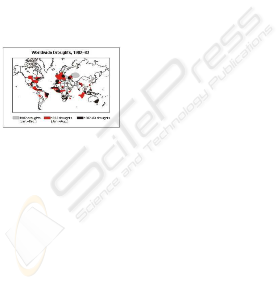
To explore the difference for information extrac-
tion from the combined patterns and the simple pat-
tern, we display a world drought map for the 1982-
1983 El Ni
˜
no episode in Figure 5 (NDMC (National
Drought Mitigation Center), 2006) because the NDVI
dataset used here spans the 1982-1992 period. Please
note that the correlation selection in our case is based
on a positive correlation coefficient while the val-
ues of SOI associated with El Ni
˜
no are negative.
Therefore, in the spatial patterns based on an NDVI
anomaly (Figres 2–4), positive values are actually as-
sociated with a negative NDVI anomaly due to ENSO,
which in return, is associated with the drought pat-
terns in Figure 5.
Figure 5: World drought pattern during the 1982-1983 El
Ni
˜
no episode (from the web site of National Drought Mit-
igation Center (NDMC (National Drought Mitigation Cen-
ter), 2006)).
The simple PCA pattern (Figure 2) does capture
drought patterns, but in large scale only, such as
droughts in the Amazon area, southern Africa, and
Australia in the 1982-1983 period. However, the
shapes and sizes of the drought patterns are difficult
to compare with the simple PCA pattern. In contrast,
the combined patterns from the selection algorithm
applications on standard PCA and KPCA capture the
details such as the curvature in the drought patterns in
the continental US for the 1983 drought. The com-
bined KPCA pattern also shows good agreement on
the drought patterns in western Africa around Ivory
Coast. The drought pattern in Malaysia and Borneo
Island (around 112E longitude near the Equator) in
the South & East Asia region is evident in the com-
bined patterns from both standard PCA and KPCA,
but they are not exhibited in the simple PCA pattern.
Another apparent improvement from the combined
KPCA spatial pattern is that the drought in Europe
is more accurately identified in contrast to the simple
PCA pattern.
5 DISCUSSION AND
CONCLUSIONS
From a data decomposition perspective, PCA as well
as KPCA are data adaptive methods. That means
that the bases for the decomposition are not chosen
a priori, but are constructed from the data. In the
standard linear PCA case, the orthogonality condition
on the spatial patterns and the uncorrelated condition
on temporal components guarantee the uniqueness of
the decomposition. Additional freedoms introduced
by the implicit nonlinear transformation make the
uniqueness condition invalid, and the KPCA results
depend on the nonlinear structure implicitly described
by the kernel. As a result, different kernels should be
tested before significant results can be discovered be-
cause the underlying nonlinear structure can only be
picked up by a kernel with a similar structure.
In a broad sense, principal component analysis de-
scribes the co-variability among multivariate obser-
vations. The definition of the co-variability between
two observations actually determines the core struc-
ture one may expect from the result. The most com-
monly used definition is covariance or correlation be-
tween points defined in either object space or vari-
able space (Krzanowski, 1988). In KPCA applica-
tion, if we do not consider the process as a mapping
from input space into the feature space, we can treat
the “kernel trick” as another definition of the pair-
wise co-variability. However, this definition of the
co-variability can only be implemented on data points
defined for each observation. That is, the KPCA is
applied to object space only. This results in the eigen-
value problem for KPCA being always on a matrix of
size N ×N, even when M, the number of variables or
geolocations in earth science applications is smaller
than N. Since the mapping function Φ is never de-
termined in the procedure, the computationally effi-
cient SVD procedure cannot be used either, because
the data matrix in feature space, D
Φ
, is not known.
The pair-wise co-variability is actually a measure
of the pair-wise proximities. Therefore, KPCA can
be understood in a broad sense as a general means
to discover “distance” or “similarity (dissimilarity)”
based structure. That is why most dimension re-
duction algorithms such as Multidimensional Scal-
ing (MDS) (Cox and Cox, 2000), Locally Linear
Embedding (LLE) (Roweis and Saul, 2000), and
Isomap (Tenenbaum et al., 2000) can be related to
KPCA algorithm (Ham et al., 2004).
In conclusion, the KPCA algorithm is recast in
the notation of PCA commonly used in earth science
communities and is used for NDVI data. To over-
come the problems of KPCA applications in earth sci-
ences, namely the overwhelming numbers of compo-
nents and lack of quantitative variance description,
A PATTERN SELECTION ALGORITHM IN KERNEL PCA APPLICATIONS
201

a new spatial pattern selection algorithm based on
correlation scores is proposed here. This selection
mechanism works both on standard PCA and KPCA,
and both give superior results compared to the tradi-
tional simple PCA pattern. In the implementation ex-
ample with NDVI data and the comparison with the
global drought patterns during the 1982-1983 El Ni
˜
no
episode, the combined patterns show much better
agreement with the drought patterns on details such
as locations and shapes.
REFERENCES
Cox, T. F. and Cox, M. A. (2000). Multidimensional Scal-
ing. Chapman & Hall.
CPC (Climate Predication Center/NOAA)
(2006). (STAND TAHITI - STAND DAR-
WIN) SEA LEVEL PRESS ANOMALY.
http://www.cpc.ncep.noaa.gov/data/indices/soi
(Last accessed on Feb. 5, 2006).
Cracknell, A. P. (1997). The Advanced Very High Resolu-
tion Radiometer. Taylor & Francis Inc.
Emery, W. J. and Thomson, R. E. (2001). Data Analysis
Methods in Physical Oceanography. Elsevier.
GES DISC (NASA Goddard Earth Sciences (GES)
Data and Information Services Center (DISC))
(2006). Pathfinder AVHRR Land Data.
ftp://disc1.gsfc.nasa.gov/data/avhrr/Readme.pal
(Last accessed on Feb. 9, 2006).
Haddad, R. A. and Parsons, T. W. (1991). Digital Sig-
nal Processing: Theory, Applications, and Hardware.
Computer Science Press.
Ham, J., Lee, D., Mika, S., and Sch
¨
olkopf, B. (2004). Ker-
nel View of the Dimensionality Reduction of Mani-
folds. In Proceedings of the 21st International Con-
ference on Machine Learning.
Hastie, T. and Stuetzle, W. (1989). Principal Curves. Jour-
nal of the American Statistical Association, 84:502–
516.
Holmes, P., Lumley, J. L., and Berkooz, G. (1996). Tur-
bulence, Coherent Structures, Dynamical Systems and
Symmetry. Cambridge University Press.
Kramer, M. (1991). Nonlinear Principal Component Anal-
ysis Using Autoassociative Neural Networks. AIChE
J., 37(2):233–243.
Krzanowski, W. J. (1988). Principles of Multivariate Anal-
ysis: A User’s Perspective. Oxford University Press.
Li, Z. and Kafatos, M. (2000). Interannual Variability of
Vegetation in the United States and Its Relation to
El Ni
˜
no/Southern Oscillation. Remote Sensing of En-
vironment, 71(3):239–247.
Lorenz, E. N. (1959). Empirical orthogonal functions and
statistical weather prediction. Final Report, Statistical
Forecasting Project, 1959; Massachusetts Institute of
Technology, Dept. of Meteorology, 29–78.
Mika, S., Sch
¨
olkopf, B., Smola, A., M
¨
uller, K.-R., Scholz,
M., and R
¨
atsch, G. (1999). Kernel PCA and De-
noising in Feature Spaces. In Kearns, M. S., Solla,
S. A., and Cohn, D. A., editors, Advances in Neural
Information Processing Systems 11, pages 536 – 542,
Cambridge, MA. MIT Press.
Monahan, A. H. (2001). Nonlinear Principal Component
Analysis: Tropical IndoPacific Sea Surface Temper-
ature and Sea Level Pressure. Journal of Climate,
14(2):219–233.
NDMC (National Drought Mitigation Cen-
ter) (2006). What is Drought?
http://www.drought.unl.edu/whatis/elnino.htm (Last
accessed on Feb. 8, 2006).
Philander, S. G. (1990). El Ni
˜
no, La Ni
˜
na, and the Southern
Oscillation. Academic Press.
Ropelewski, C. and Jones, P. (1987). An Extension of the
Tahiti–Darwin Southern Oscillation Index. Monthly
Weather Review, 115(9):2161–2165.
Roweis, S. and Saul, L. (2000). Nonlinear Dimensional-
ity Reduction by Locally Linear Embedding. Science,
290(22 December 2000):2323–2326.
Sch
¨
olkopf, B., Burges, C., and Smola, J. (1999a). Advances
in Kernel Methods: Support Vector Learning. MIT
Press.
Sch
¨
olkopf, B., Mika, S., Burges, C., Knirsch, P., M
¨
uller, K.-
R., R
¨
atsch, G., and Smola, A. (1999b). Input Space
vs. Feature Space in Kernel-Based Methods. IEEE
Transactions on Neural Networks, 10(5):1000–1017.
Sch
¨
olkopf, B., Smola, A., and M
¨
uller, K.-R. (1998). Non-
linear Component Analysis as a Kernel Eigenvalue
Problem. Neural Computation, 10(5):1299–1319.
Tan, J. (2005). Applications of Kernel PCA Methods to Geo-
physical Data. George Mason University. PhD Thesis.
Tan, J., Yang, R., and Kafatos, M. (2006). Kernel PCA
Analysis for Remote Sensing Data. In 18th Confer-
ence on Climate Variability and Change. American
Meteorological Society. Paper P1.5, Altanta, GA, CD-
ROM.
Tenenbaum, J., de Silva, V., and Langford, J. (2000).
A Global Geometric Framework for Nonlinear Di-
mensionality Reduction. Science, 290(22 December
2000):2319–2323.
Thompson, D. W. J. and Wallace, J. M. (2000). Annular
Modes in the Extratropical Circulation. Part I: Month-
to-Month Variability. Journal of Climate, 13(5):1000–
1016.
Von Storch, H. and Zwiers, F. W. (1999). Statistical Analy-
sis in Climate Research. Cambridge University Press.
Wallace, J. M., Smith, C., and Bretherton, C. S. (1992). Sin-
gular Value Decomposition of Wintertime Sea Surface
Temperature and 500-mb Height Anomalies. Journal
of Climate, 5(6):561–576.
ICSOFT 2006 - INTERNATIONAL CONFERENCE ON SOFTWARE AND DATA TECHNOLOGIES
202
