SURFACE CONSTRUCTION USING TRICOLOR

MARCHING CUBES

Shaojun Liu, Jia Li

Oakland University

Rochester, MI 48309, USA

Xiaojun Jing

Beijing University of Posts and Telecommunications

No. 10 Xi Tu Cheng Rd, Beijing 100876, China

eywords:

Marching cubes, 3D surface construction.

Abstract:

This paper presents a generalized marching cubes (MC) method for 3D surface construction. Existing MC

methods require the sample values at cell vertices to be different from the threshold or modify them otherwise.

The modiﬁcation may introduce topological changes to the constructed surface. The proposed Tricolor MC

method allows cell vertices with sample values which equal the threshold to lie on the surface. It constructs the

surface patches by exhausting the Eulerian circuits in the cells without changing sample values. The simulation

results show that the TMC method better preserves the topology of the surfaces that pass through cell vertices

and gives good results in other general cases.

1 INTRODUCTION

Three dimensional (3D) surface construction is a

widely studied topic in computer graphics and com-

puter vision. Polygonal representation of 3D surface,

or mesh, is extensively used in rendering on graph-

ics hardware, texture mapping, and shape analysis.

The marching cubes (MC) method is the most pop-

ular method to generate isosurface on volumetric data

at uniform grids. Proposed by Lorensen and Cline in

1987, MC method is fast in extracting high resolu-

tion isosurfaces and simple to implement (Lorensen

and Cline, 1987). However, the original MC method

has problems such as topology inconsistency and rep-

resentation inaccuracy. Since then a variety of MC

methods have been proposed for improvements.

Nielson and Hamann proposed an asymptotic de-

cider to solve the face ambiguity which happens in

a cube face with two diagonally opposite vertices

marked positive and the other two marked nega-

tive (Nielson and Hamann, 1991). Chernyaev used

33 conﬁgurations to eliminate the internal ambigu-

ity which occurs in the interior of a cube (Chernyaev,

1995). Ho et al. proposed CMS method to preserve

sharp features (Ho et al., 2005).

One of the original MC assumptions is not ad-

dressed by later variations, which assumes the cell

vertices lie either inside or outside the surface, not

on the surface. It meets a problem when isocontours

such as level set pass through cell vertices. To elide

this problem, existing MC methods modify the sam-

ple values that equal threshold. This modiﬁcation,

however, may introduce obvious topological changes

in some cases as shown in the latter part of the paper.

This paper proposes a more general MC method

that does not modify the sample values. It constructs

surface by ﬁnding Eulerian circuits in the cell. The

paper is organized as following. In Section 2, the

background for MC method is brieﬂy introduced. In

Section 3, we propose the new MC method and intro-

duce the surface construction procedure. The exper-

imental results are presented in Section 4. Section 5

concludes the paper.

2 BACKGROUND

The output of the marching cube algorithm is a mesh

representing the 3D surface. A mesh M is a pair

(K, V ), where K is a simplicial complex represent-

ing the connectivity of the vertices, edges and faces,

thus determining the topological type of the mesh, and

V = {v

,...,v

},v

∈

is a set of vertex coordi-

nates deﬁning the shape of the mesh in 

The input of the MC algorithm is volumetric data,

which has sample value associated with each grid

point. The samples at cell vertices are thresholded

before isosurface extraction. Hereafter the sample

319

Liu S., Li J. and Jing X. (2006).

SURFACE CONSTRUCTION USING TRICOLOR MARCHING CUBES.

In Proceedings of the First International Conference on Computer Graphics Theory and Applications, pages 319-324

DOI: 10.5220/0001350703190324

 SciTePress

−

(a) (b) (d)(c)

−

−−

−

−−

−

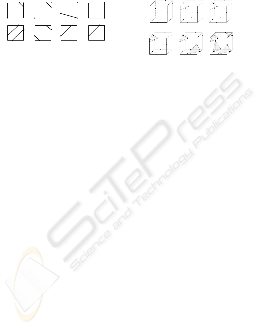
Figure 1: Topological changes caused by sample value

modiﬁcation. In each subﬁgure, the ﬁgure on the top shows

the original sample values, while the ﬁgure at the bottom

shows the possible topological change.

value is referred as that minus threshold. And we

call the cell vertex with positive/negative/zero sam-

ple value positive/negative/zero cell vertex re-

spectively. Existing MC methods do not allow cell

vertices lie on the surface, or zero cell vertices. Un-

der this assumption, the surface is limited to intercept

the cell in 2

= 256 ways since each of the eight

cell vertices can lie either inside or outside the sur-

face. It is equivalent to coloring the eight cell vertices

with two colors. Hence we call existing MC methods

bicolor methods. By exploiting the symmetries in the

256 ways, Lorensen et al. summarized the cases into

15 patterns in the original MC method (Lorensen and

Cline, 1987).

To hold this assumption, existing bicolor MC meth-

ods have to modify the zero sample value in prac-

tice. For example, as level set may pass through grid

points, Han et al. change the sample value at such grid

points from zero to negative (Han et al., 2003). This

kind of modiﬁcation may introduce obvious topolog-

ical changes, which is shown in Fig. 1. The thick line

in the ﬁgure represents the interception of surface and

cell face. Modiﬁcation on sample value changes the

original cell face into ambiguous faces as shown in

(a) and (b). And the interceptions become completely

different after modiﬁcations on (c) and (d). Secondly,

the isosurface extracted should be neutral with posi-

tive and negative data samples. In other words, the

isosurface should not change if we multiply the sam-

ple data with −1. Modifying the sample value, how-

ever, can lead to two different topological results for

the same set of data as shown in the experiment sec-

tion of this paper. Thirdly, modifying sample value

may introduce nonexistent face as shown in the ex-

periments.

This defect is regarded as a technical problem in

(Gelder and Wilhelms, 1994), and one of the several

major artifacts in most existing isocontour software

(Han et al., 2003). One of the reasons that existing

bicolor MC methods elide this problem is too many

cases are introduced without this assumption. If the

sample at cell vertex is allowed to be zero, each of the

eight cell vertices has three instead of two possible

positions relative to the surface, i.e. inside, outside

(1) (2) (3)

(4) (5) (6)

Figure 2: An example of one possible way to ﬁnd 4 patches

edge by edge in a cell with 12 vertices.

or on the surface. Thus the surface intercepts the unit

cube in a total of 3

= 6561 ways. It is equivalent to

coloring cell vertices with three colors. We name our

method tricolor MC (TMC) to reﬂect this character.

To enumerate all these ways and reduce the symme-

tries manually, as what has been done in (Lorensen

and Cline, 1987), is extremely tedious and error-prone

to human. In the following sections, we will eliminate

this assumption to include zero cell vertices without

modiﬁcation.

3 SURFACE CONSTRUCTION

For the convenience of discussion, we deﬁne patch

as the close interception of the isosurface and a cell, a

polygon formed by connecting the surface mesh ver-

tices. A patch edge is the interception of the surface

with a cell face, whose end points are two adjacent

surface mesh vertices on the cell edge. The degree

of surface vertex is the number of patch edges inci-

dent on the vertex. Since we are only interested on the

patch edges in one cell, hereafter the vertex degree ac-

tually refers to the degree in one cell. As mentioned

in Section 2, the cell may hold the patches in 6561

ways if taking zero cell vertices into consideration.

Instead of enumerating all these cases, we go back to

two dimensions to examine the ways of the intercep-

tion of isosurface and one cell face, or the patch edges.

As the patch is enclosed by patch edges, it forms an

Eulerian circuit, a graph cycle which uses each graph

edge exactly once. It suggests ﬁnding the patches in

the cell by ﬁnding the Eulerian circuits. We start from

any of the surface vertex, ﬁnd one patch edge incident

on it if possible, and continue with the surface vertex

that is the other endpoint of the patch edge until we

return to the original vertex. After one Eulerian cir-

cuit, or a patch, is completed, repeat the process until

all the patch edges in the cell have been visited. Then

we ﬁnd all the patches in the cell. An example of one

possible way to ﬁnd 4 patches edge by edge by within

one cell is illustrated in Fig. 2.

As more than two surface vertices may lie on a

GRAPP 2006 - COMPUTER GRAPHICS THEORY AND APPLICATIONS

320

(13)

(1)

+−

(3)

0−

(5)

−−

(6)

(4)

(7) (8)

(2)

(9)

−0

(11)(10)

−

−+ 00

(12)

−

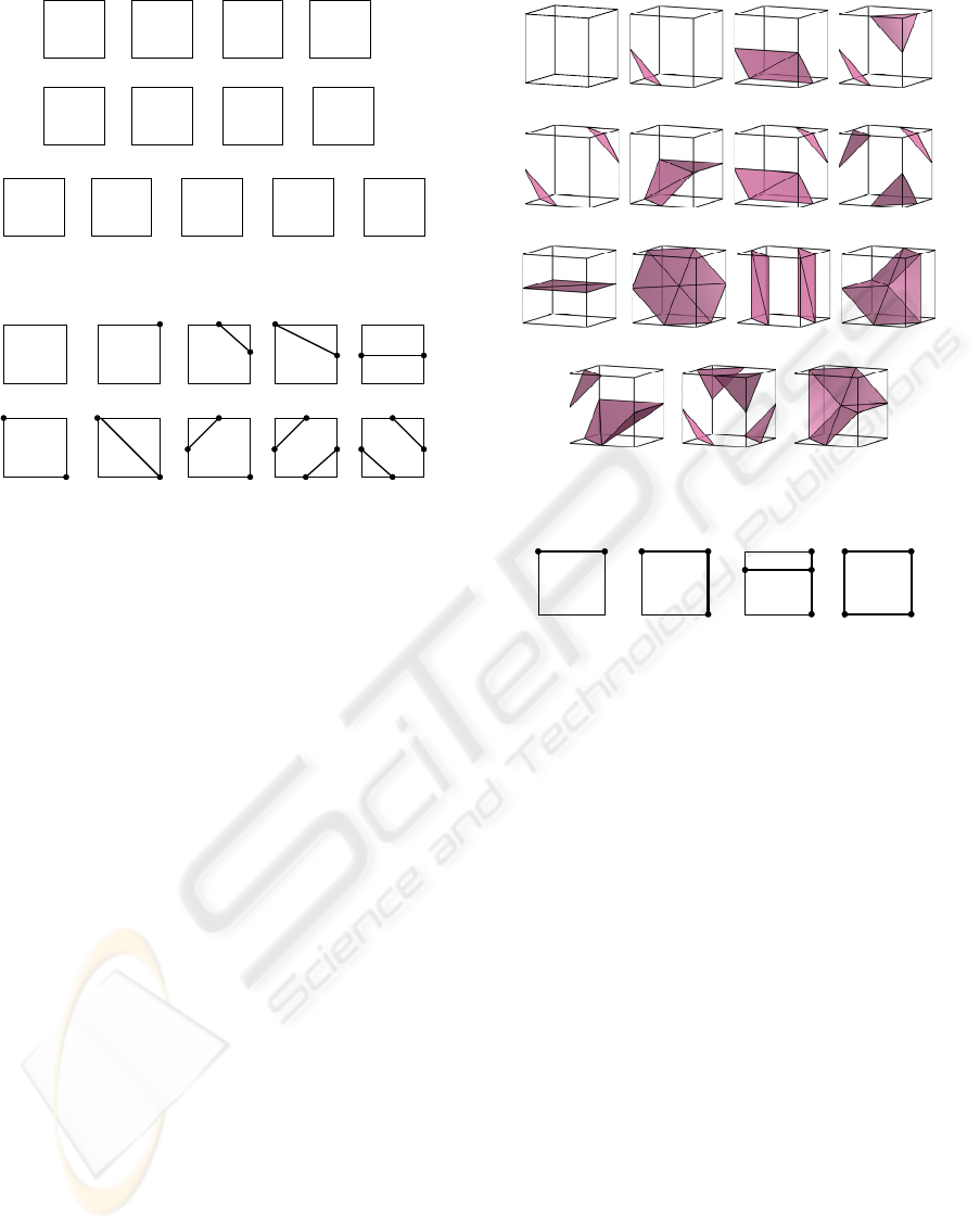
Figure 3: 13 cases of squares with zero cell vertices.

(9)

0−

(5)

(1) (2)

(3)

−

−−

(6)

(7) (10)

+−

(13.a)

−+

(13.b)

−

0−

Figure 4: 10 cases out of the original 13 cases in Fig. 3 with

zero cell vertices and their corresponding patch edges.

cell face, there are multiple ways to deﬁne the patch

edges. And the resulted patches in the cell would be

completely different. So we need to count how many

ways to deﬁne the edges on a cell face and make our

choice. Banks et al. counted the cases to produce

substitopes in the MC method (Banks and Linton,

2003). They enumerated 13 distinct cases in two di-

mensions with zero cell vertices as shown in Fig 3, in

which symmetries between positive and negative cell

vertices have been eliminated. Many of these cases,

however, allow ambiguous ways to connect the patch

edges. Various methods have been proposed to solve

the ambiguities. The bilinear interpolation over the

cell face is adopted to solve the ambiguity problem in

our study,

φ(u, v)=φ

(1 − u)(1 − v)+φ

(1 − u)v

+φ

u(1 − v)+φ

(1)

where φ(u, v) stands for the value at logical coordi-

nates (u, v) on the cell face (Nielson and Hamann,

1991). This bilinear interpolation solves most cases

as shown in Fig. 4. The choice of ambiguous sub-

cases 13.a and 13.b is made according to the method

proposed in (Nielson and Hamann, 1991). Note that

the proposed method does not address internal ambi-

guity since it only allows patch edges on the cell face.

Case 1, 3, 6, 13.a and 13.b of Fig. 4 correspond

to all the 15 cases in the original MC method. To

show that the proposed method cover all the cases

of the original MC methods, we use the 15 cases in

the original MC method as input of TMC method and

get the same patches as the original MC method in

Fig. 5, though the triangulation is different. TMC

(0) (1) (2) (3)

(4) (5) (6) (7)

(8) (9) (10) (11)

(12) (13) (14)

Figure 5: 15 cases in original MC method covered by TMC.

(11)

−00

(12)

(4)

(8)

Figure 6: Bilinear Interpolation of case 4, 8, 11 and 12 in

Fig. 3.

method also generates the same results for all the pos-

sible conﬁgurations with ambiguous faces as those in

(Nielson and Hamann, 1991). Due to page limit, we

do not list the result here.

However, ambiguities in case 4, 8, 11 and 12 of Fig.

3 are not solved well by bilinear interpolation, which

is shown in Fig. 6. In case 11, one patch edge inter-

cepts with the other between its endpoints, resulting

in discontinuous surface. And too little information

is available to decide the patch edges at the border of

a cell face, which is called border edge. To ensure

the patch edge is on the border of two regions with

different sign, both cell faces incident on the possible

border edge need to be checked. The cases in Fig.

4 can be used to solve these ambiguities if the two

adjacent cell faces are ”merged” into one. In the fol-

lowing, we enumerate the combinations of case 4, 8,

11 and 12 with the 13 cases of Fig. 3.

First we list the combinations without case 12 as

shown in Fig. 7. For example, case 4 of Fig. 3 has

ﬁve sub-cases from 4.a to 4.e in Fig. 7 with regard

to the cell face incident on the possible border edge.

And the ambiguous sub-cases 11.e.1 and 11.e.2 are

solved in the same way as 13.a and 13.b of Fig. 4. As

for the sub-cases 11.c.1 and 11.c.2, we choose 11.c.1

if the sum of absolute sample values at positive cell

vertices is greater than that at negative cell vertices,

SURFACE CONSTRUCTION USING TRICOLOR MARCHING CUBES

321

(8.h)

−0

−

(11.b,8.c) (11.c.1)

−

(11.c.2) (11.d,8.d)

−

(4.a)

+−

(4.b,8.a) (4.c,11.a)

0−

−

(4.d,8.b) (4.e)

(11.e.1)

(8.e) (8.f)(11.e.2) (8.g)

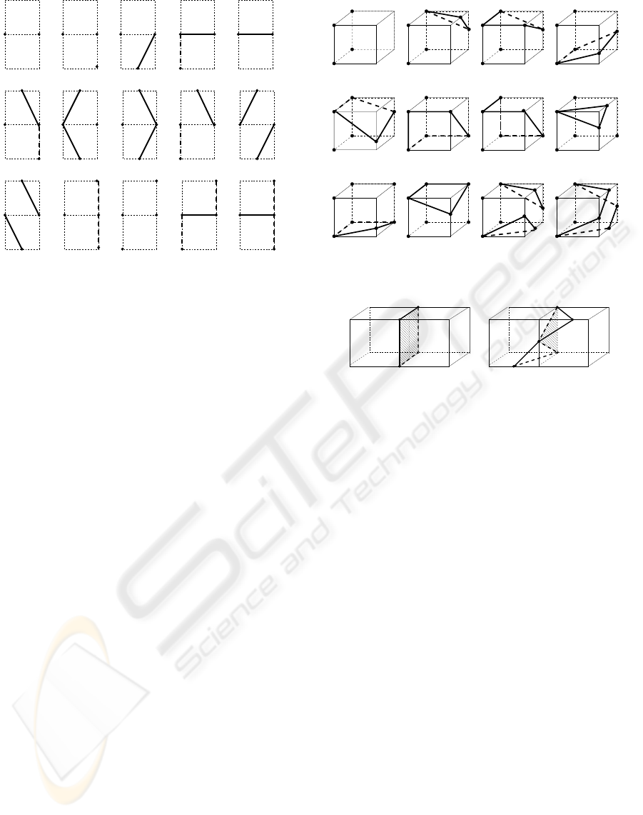
Figure 7: Solving ambiguities in case 4, 8 and 11 of Fig. 3.

Solid line stands for the patch edge while dotted line for the

undecided patch edge.

and 11.c.2 otherwise. As each of the sub-cases of case

8 in Fig. 7 has two possible border edges, we need to

check the two adjacent cell faces incident on the two

possible border edges.

As for the combinations with case 12 of Fig. 3, the

other eight cell vertices in the cell have only 13 dis-

tinct conﬁgurations of Fig. 3 due to symmetry. So

we can enumerate all the 13 conﬁgurations and gen-

erate patch edges accordingly. To use the results in

Fig. 7, we ”shrink” the cell face of case 12 into a bor-

der edge. Fig. 8 shows the patch edges for the twelve

sub-cases of case 12 of Fig. 3 in 3D. Note sub-case

12.a represents the conﬁgurations in which the other

eight vertices in the cell are the cases of 1, 2, 4, 7, 8 or

12 of Fig. 3. As for the ambiguous sub-cases 12.d.1

and 12.d.2, 12.e.1 and 12.e.2 or 12.g.1 and 12.g.2,

we choose 12.d.1, 12.e.1 or 12.g.1 if the sum of ab-

solute sample value at positive cell vertices is greater

than that at negative cell vertices, and 12.d.2, 12.e.2

or 12.g.2 otherwise. And the ambiguous sub-cases

12.h.1 and 12.h.2 are solved in the same way as 13.a

and 13.b in Fig. 4.

By solving the 13 tricolor cases of Fig. 3 accord-

ing to Fig. 4, Fig. 7 and Fig. 8, we can decide patch

edges for all the 6561 cases in 3D. But we still need

to ensure that TMC method can ﬁnd all the patches by

searching the Eulerian circuits in the cell. The condi-

tion of Eulerian circuits is no surface vertex with odd

degree. We show brieﬂy in the following that the de-

gree of surface vertex in one cell is either zero or two.

And the surface vertex with zero degree is isolated

and simply ignored.

Firstly, it is easy to verify the degree of surface ver-

tex, which is not zero cell vertex, is two. And the de-

gree of surface vertex in Fig. 8 is either zero or two.

Secondly, we show that the degree of surface vertex

−

(12.a)

0/+

−

(12.d.2)

−

(12.g.1)

0/+

(12.b)

−

(12.e.1)

−

(12.g.2)

−

(12.c)

−

(12.e.2)

−

(12.h.1)

−

(12.d.1)

−

(12.f)

−

(12.h.2)

Figure 8: Solving ambiguities in case 12 of Fig. 3.

−

(a) Case 12 of Fig. 3

−

(b) Case 11 of Fig. 3

Figure 9: Insert one patch between two adjacent cells rep-

resented by the ﬁlled region.

is at most two for the cases with zero cell vertices in

Fig. 4 and Fig. 7. In Fig. 4, if one zero cell ver-

tex connects to three patch edges like case 5 or 9, it

will cause a contradiction, in which the cell vertices at

the two sides of one patch edge are of the same sign.

In Fig. 7, we only need to check the degree of zero

cell vertex that possibly connect more than one patch

edge. Since only two cell vertices are not known in

Fig. 7, we get the degree is two by enumerating the

nine combinations of the two unknown cell vertices

in sub-cases 4.d, 11.b, 11.c.1, 11.c.2, 8.e, 8.g and 8.h.

Finally we show that the degree of zero cell vertex is

not one. We only need to check the zero cell vertex

that connects only one patch edge in Fig. 4 and Fig.

7. From case 5 and 9 of Fig. 4, the zero cell ver-

tex connects to only one patch edge on one cell face

if its two adjacent cell vertices are of different sign.

Similarly it connects to at least one patch edge in its

other adjacent cell faces, if its third adjacent cell ver-

tex (not displayed) is positive or negative. If its third

adjacent cell vertex is zero, only two other unknown

cell vertices (not displayed) affect its degree. We get

the degree is two by enumerating the nine combina-

tions of the two unknown cell vertices. In Fig. 7, the

degree of zero cell vertex in sub-cases 4.c, 4.e, 11.e.1,

11.e.2 is two since its two adjacent cell vertices are of

different sign. And we get the degree is two by enu-

merating sub-case 4.d, 11.b, 11.d, 8.e, 8.g and 8.h.

As the cell face of case 12 of Fig. 3 is shared by

GRAPP 2006 - COMPUTER GRAPHICS THEORY AND APPLICATIONS

322

−

−−

−

−−

−

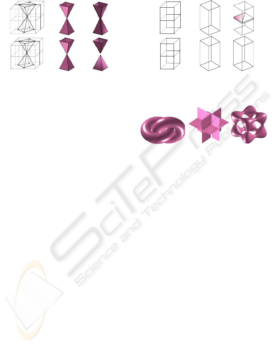
(a) Original Topology (b) TMC (c) Bicolor MC

Figure 10: Topologies comparison between TMC and the

Lewiner’s MC implementation on cases 2 in Fig. 4.

two adjacent cells, if it separates two regions of dif-

ferent sign, we need to insert a patch between the two

adjacent cells as shown in Fig. 9(a). Moreover, as

the cell face of case 11 may result in different patch

edges in two adjacent cells, a new patch is also needed

as shown in Fig. 9(b). Note these patches inserted

between adjacent cells do not affect the previous con-

clusion about the vertex degree in the cell.

The orientation of patch vertices is adjusted to keep

the patch normal pointing outward the surface consis-

tently. Once all the patches are found, we complete

the whole front surface. To get the triangulate mesh,

we triangulate each patch by using one vertex as the

common triangle vertex. To avoid self intersection be-

tween patches within one cell (Gelder and Wilhelms,

1994), we add a new vertex, which is the average of

other vertices, as the common triangle vertex for poly-

gons with more than ﬁve edges.

Banks and Linton also counted the tricolor cases

in three dimensions in MC method by numerical al-

gorithms (Banks and Linton, 2003). They found 147

cases out of the original 6561 cases. However, it is

unrealistic to verify this result by hand. Enumerating

all the ambiguous cases for these 147 cases is also a

tedious task.

Another advantage of the TMC method is that 2D

contours have already been generated by patch edges

within each patch. By collecting the patch edges on

every plane, we can get the 2D contour at speciﬁed

position. Ho et al. also constructed surface by ﬁnding

2D segments in their CMS method (Ho et al., 2005).

But the CMS method does not consider the zero cell

vertex, hence it inherits the topological artifacts of the

bicolor algorithms.

4 EXPERIMENTAL RESULTS

AND ANALYSIS

To show the advantage of the proposed TMC method,

we test it over the cases shown in Fig. 10 and com-

−

−−

(a) Original Topology (b) TMC (c) Bicolor MC

Figure 11: Topologies comparison between TMC and the

Lewiner’s MC implementation on case 12 in Fig. 3.

(a) Two torus (b) Case (c) Blooby

Figure 12: Examples constructed by TMC.

pare it with an existing bicolor MC method imple-

mented by Lewiner et al. (Lewiner et al., 2003).

Lewiner’s implementation is based on Chernyaev’s

technique, to solve the ambiguity problem on the cell

face (Chernyaev, 1995). It modiﬁes the zero sample

value at cell vertex to a small positive value. For the

case shown in top row in Fig. 10, Lewiner’s method

reports eight times of case 2 of Fig. 5 and gener-

ates 16 triangles. When the data are multiplied by

−1 as shown in the bottom case in Fig. 10, the pro-

posed TMC method consistently preserves the orig-

inal topology, while Lewiner’s method reports eight

times of case 1 of Fig. 5 and generates 8 triangles. To

illustrate, we enlarge its small positive value to 0.05

and get the result in Fig. 10. Note this enlargement

does not change its topology or the number of trian-

gles generated.

On case 12 of Fig. 3, Lewiner’s MC implementa-

tion outputs two planes for the top case in Fig. 11.

But it generates no plane when the data samples are

multiplied by −1 as the bottom case in Fig. 11. In

comparison, TMC gives no plane consistently since

these zero cell vertices are not the boundary of two

regions with different signs.

To illustrate TMC can extract the isosurface cor-

rectly, we synthesize volume data with known under-

lying functions and use them as the input (Lewiner

et al., 2003). The results are accordant with the un-

derlying functions as shown in Fig. 12. We also

test the proposed algorithm on volumetric data with

unknown underlying surface function. A series of

CT lung scans have been downloaded from the Na-

SURFACE CONSTRUCTION USING TRICOLOR MARCHING CUBES

323

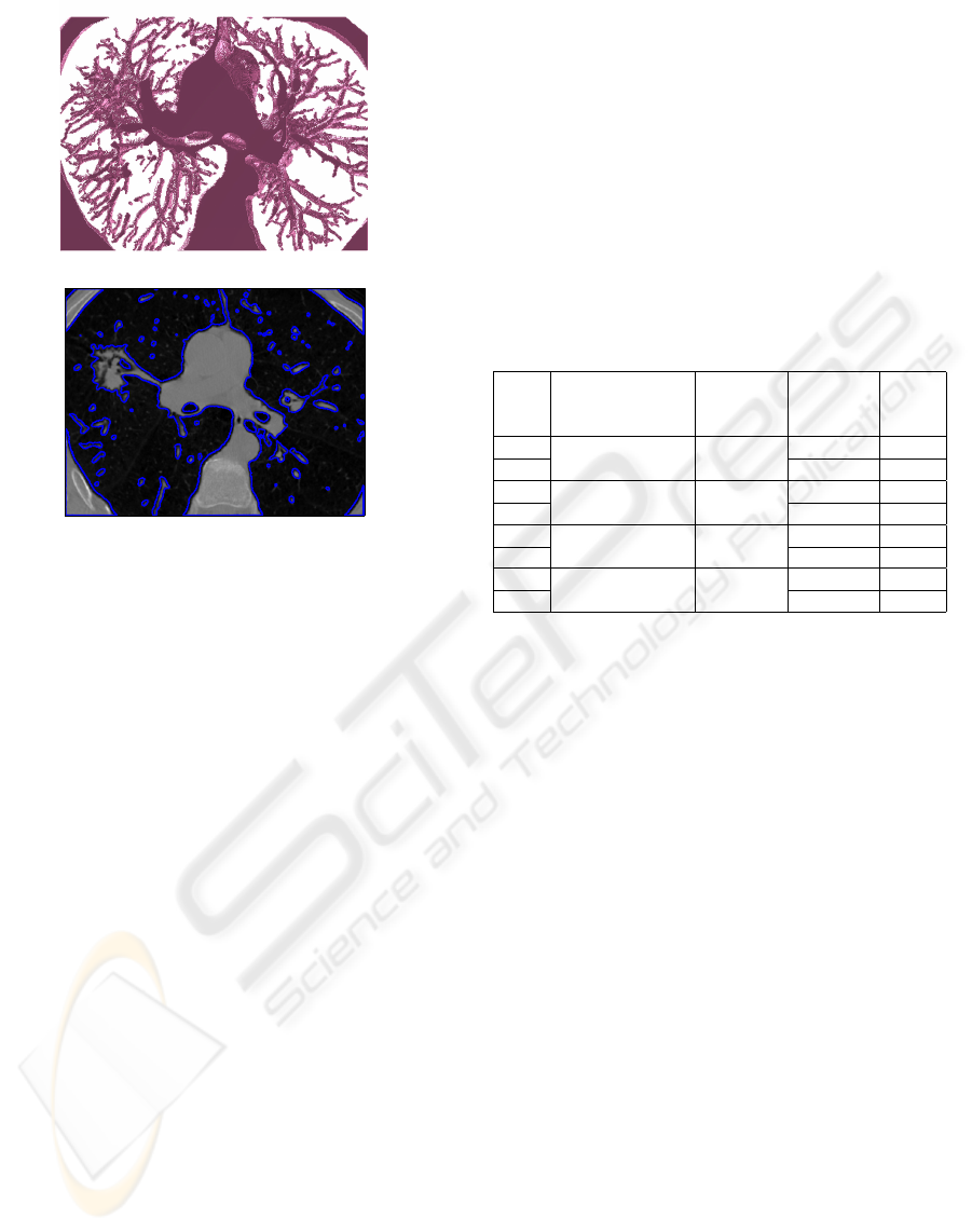
(a) 3D surface

(b) 2D contour

Figure 13: Internal lung structures constructed from seg-

mentation results.

tional Cancer Institute [LIDC]. First the 3D image in

the region of interest (ROI) is segmented by level set

method. Then TMC is used to construct surface from

the level set results. Fig. 13(a) shows the results on

the ROI with 290×380×62 voxels. As mentioned, the

2D contours can be conveniently collected during ex-

tracting isosurface by TMC method as shown in Fig.

13(b), while tremendous efforts are needed for gener-

ating 2D contours in most existing MC methods. In

the image, the thin structures like lung bronchia and

ﬁne surface details are well captured. And the results

have been validated by experienced physicians.

We also compare the running time of TMC method

with Lewiner’s MC implementation as shown in Table

1. TMC method is a little bit slower than Lewiner’s

method because of the added cases. It is still a fast

algorithm, which can generate 4 million triangles in

8.5 seconds in one experiment. The table shows that

the number of zero cell vertices are about 1% to 4% of

that of the resulted triangles. All the experiments are

carried out on a Pentium IV 3.2GHZ processor with

1G RAM.

5 CONCLUSION

We propose a tricolor marching cubes (MC) method

for 3D surface construction. Existing bicolor MC

methods do not allow cell vertices whose sample val-

ues equal threshold, or zero cell vertices. Modifying

sample value at such vertices may change the topol-

ogy of original surface. The proposed TMC method

allows the third ”color”, i.e. zero value prevail cell

vertices after thresholding. It constructs the isosur-

face by ﬁnding Eulerian circuits in the cells. Com-

paring with the existing MC methods, the proposed

method has the following advantages. First it best pre-

serves the original topology since it does not modify

sample values at cell vertices. Secondly it avoids enu-

merating a large number of the cases introduced by

zero cell vertices. Thirdly it generates 2D contours

of the surface automatically. Simulation results show

that TMC method preserves topology better than ex-

isting MC methods on contacting surfaces and is an

efﬁcient method in constructing 3D surfaces.

Table 1: Running time of TMC and MC method.

Dimension Zero

Cell

Vertices

Triangles Time

(s)

200 × 360 × 28 7407

260545 0.469

TMC 267167 0.718

290 × 380 × 62 22081

548321 1.375

TMC 546660 1.75

512 × 512 × 28 16054

1118504 2.063

TMC 1137072 2.578

512 × 512 × 59 49227

4130056 5.0

TMC 4180029 8.469

REFERENCES

Banks, D. C. and Linton, S. (2003). Counting cases in

marching cubes: Toward a generic algorithm for pro-

ducing substitopes. In IEEE Visualization 2003, pages

51–58.

Chernyaev, E. V. (1995). Marching cubes 33: Construction

of topologically correct isosurfaces. Technical Report

CN/95-17, CERN, Geneva, Switzerland.

Gelder, A. V. and Wilhelms, J. (1994). Topological consid-

erations in isosurface generation. ACM Transactions

on Graphics, 13(4):337–375.

Han, X., Xu, C., and Prince, J. (June 2003). A topology

preserving level set method for geometric deformable

models. IEEE Transactions on Pattern Analysis and

Machine Intelligence, 25(6):755–768.

Ho, C.-C., Lee, P.-L., Chuang, Y.-Y., Chen, B.-Y., and

Ouhyoung, M. (2005). Cubical marching squares:

Adaptive feature preserving surface extraction from

volume data. In EUROGRAPHICS, volume 24.

Lewiner, T., Lopes, H., Vieira, A. W., and Tavares, G.

(2003). Efﬁcient implementation of marching cubes’

cases with topological guarantees. Journal of Graph-

ics Tools, 8(2):1–15.

Lorensen, W. E. and Cline, H. E. (1987). Marching cubes:

A high-resolution 3D surface construction algorithm.

In Proceedings of the 14th annual conference on com-

puter graphics and interactive techniques, pages 163–

169.

Nielson, G. M. and Hamann, B. (1991). The asymptotic

decider: Resolving the ambiguity in marching cubes.

In Proceedings of Visualization ’91, pages 29–38.

GRAPP 2006 - COMPUTER GRAPHICS THEORY AND APPLICATIONS

324