MESH RETRIEVAL BY COMPONENTS

Ayellet Tal

∗

Department of Electrical Engineering

Technion

Emanuel Zuckerberger

Department of Electrical Engineering

Technion

Keywords:

3D shape retrieval, 3D shape matching.

Abstract:

This paper examines the application of the human vision theories of Marr and Biederman to the retrieval of

three-dimensional objects. The key idea is to represent an object by an attributed graph that consists of the

object’s meaningful components as nodes, where each node is ﬁt to a basic shape. A system that realizes this

approach was built and tested on a database of about 400 objects and achieves promising results. It is shown

that this representation of 3D objects is very compact. Moreover, it gives rise to a retrieval algorithm that is

invariant to non-rigid transformations and does not require normalization.

1 INTRODUCTION

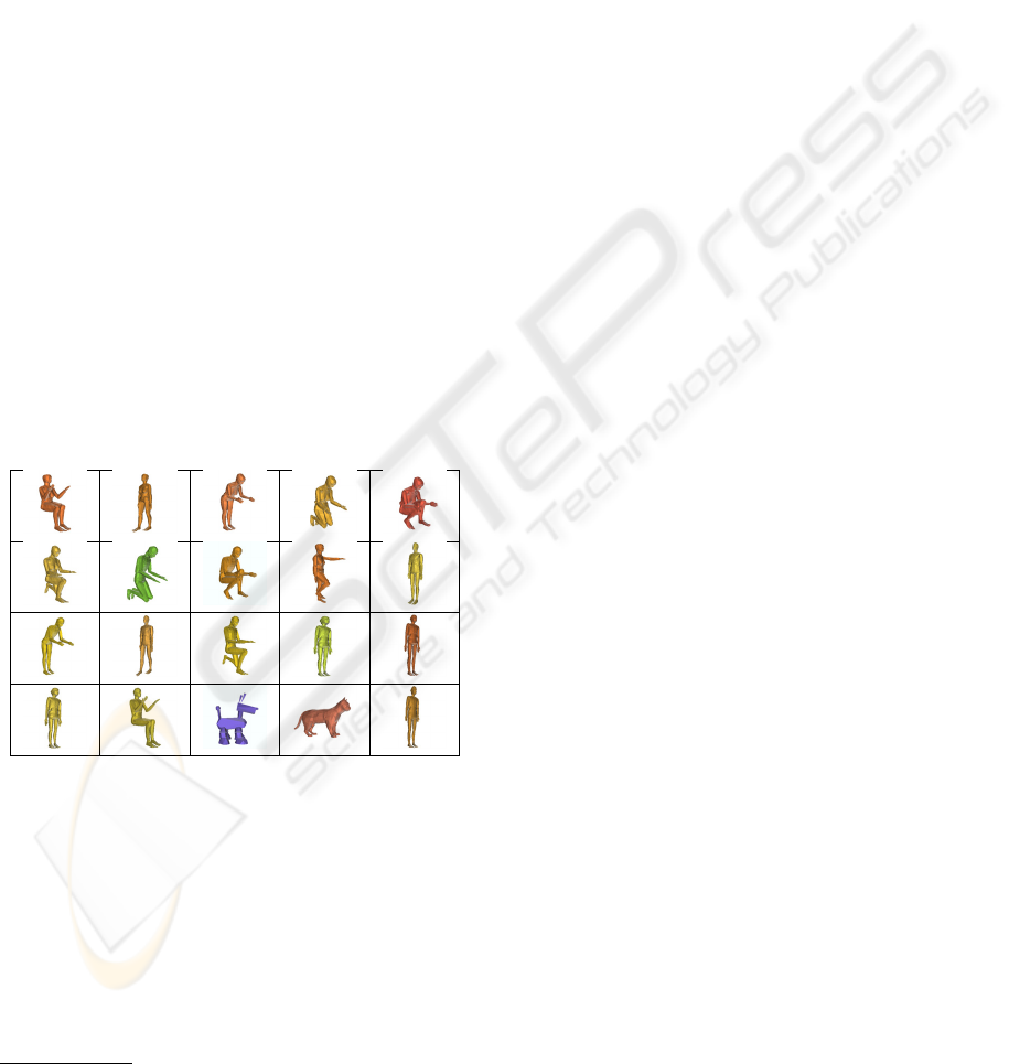
Figure 1: Retrieval of the top 20 objects similar to to the top

left-most human ﬁgure.

In his seminal work (Marr, 1982), Marr claims

that the human brain constructs a 3D viewpoint-

independent model of the image seen. This model

consists of objects and spatial inter-relations between

them. Every 3D object is segmented into primitives,

which can be well approximated by a few simple

shapes. Biederman’s Recognition-By-Components

(RBC) theory (Biederman, 1987; Biederman, 1988)

∗

This work was partially supported by European FP6

NoE grant 506766 (AIM@SHAPE) and by the Smoler Re-

search Funds.

claims that the human visual system tends to segment

complex objects at regions of deep concavities into

simple basic shapes, geons. The simple attributed

shapes along with the relations between them form

a stable 3D mental representation of an object.

The current paper proposes a retrieval approach

that attempts to succeed these theories. The key idea

is to decompose each object into its “meaningful”

components at the object’s deep concavities, and to

match each component to a basic shape. After de-

termining the relations between these components,

an attributed graph that represents the decomposition

is constructed and considered the object’s signature.

Given a database of signatures and one speciﬁc signa-

ture, the latter is compared to other signatures in the

database, and the most similar objects are retrieved.

Retrieving 3D objects has become a lively topic of

research in recent years (Veltkamp, 2001). A common

practice is to represent each object by a few prop-

erties – a signature – and base the retrieval on the

similarity of the signatures. Some signatures consist

of local properties of the shapes such as histograms

of colors and normals (Paquet et al., 2000), probabil-

ity shape distributions (Osada et al., 2001), reﬂective

symmetry (Kazhdan et al., 2003a), spherical harmon-

ics (Vranic and Saupe, 2002; Kazhdan et al., 2003b)

and more. Other papers consider global properties,

such as shape moments (Elad et al., 2001) or sphere

projection (Leifman et al., 2005). In these cases, the

objects need to be normalized ahead of time.

142

Tal A. and Zuckerberger E. (2006).

MESH RETRIEVAL BY COMPONENTS.

In Proceedings of the First International Conference on Computer Graphics Theory and Applications, pages 142-149

DOI: 10.5220/0001352001420149

 SciTePress

Our global approach is mostly related to graph-

based algorithms. The Reeb graph is a skeleton deter-

mined using a scalar function, which is chosen in this

case to be the geodesic distance (Hilaga et al., 2001).

In (Sundar et al., 2003; Cornea et al., 2005), it is pro-

posed to represent an object by its skeleton and an

algorithm for comparing shock graphs is presented.

Our approach succeeds these methods, yet differs in

several ways. First, the graphs are constructed differ-

ently, focusing on segmentation at deep concavities,

following (Marr, 1982; Biederman, 1995). Second,

each node and edge in the graph is associated with

properties, resulting in an attributed graph. Third, a

different graph matching procedure is utilized.

Our proposed signature has a few important proper-

ties. First, it is invariant to non-rigid-transformations.

For instance, given a human object, we expect its sig-

nature to be similar to signatures of other humans,

whether they bend, fold their legs or point forward,

as illustrated in Figure 1. In this ﬁgure, all the 19

humans in a database consisting of 388 objects, were

ranked among the top 21 objects, and 17 among the

top 17. Invariance to non-rigid-transformations is

hard to achieve when only geometry is considered.

Second, normalization is not required, since the

signature is a graph that is invariant to rigid transfor-

mations.

Third, the signature tolerates degenerated meshes

and noise. This is so because the object is represented

by its general structure, ignoring small features.

Finally, the proposed signature is very compact.

Thus, signatures can be easily stored and transfered.

The remaining of the paper is structured as follows.

Section 2 outlines our approach. Sections 3–4 address

the main issues involved in the construction of a sig-

natures. In particular, Section 3 discusses mesh de-

composition into meaningful components while Sec-

tion 4 describes the determination of basic shapes.

Section 5 presents our experimental results. Section 6

concludes the paper.

2 SYSTEM OVERVIEW

Given a database of meshes in a standard represen-

tation consisting of vertices and faces (e.g., VRML)

and one speciﬁc object O, the goal is to retrieve from

the database objects similar to O.

This section starts by outlining the signature com-

putation technique. This is the main contribution of

the paper and thus the next sections elaborate on the

steps involved. Then, the section brieﬂy describes the

graph matching algorithm used during retrieval.

IGNATURE COMPUTATION: Let S be an orientable

mesh.

Deﬁnition 2.1 Decomposition: S

,...S

is a de-

composition of S iff (i) ∀i,1 ≤ i ≤ k, S

⊆ S, (ii) ∀i, S

is connected, (iii) ∀i = j,1 ≤ i, j ≤ k, S

and S

are

face-wise disjoint and (iv) ∪

i=1

= S.

Deﬁnition 2.2 Decomposition graph: Given a de-

composition S

,···S

of a mesh S, a graph G(V,E)

is its corresponding decomposition graph iff each

component S

is represented by a node v

∈ V and

there is an arc between two nodes in the graph iff the

two corresponding components share an edge in S.

Deﬁnition 2.3 Attributed decomposition

graph: Given a decomposition graph G(V, E),

G =(V,E,

) is an attributed decomposition graph

is a function which assigns attributes to nodes

and

is a function which assigns attributes to arcs.

For each object in the database, its attributed de-

composition graph, the object’s signature, is com-

puted and stored. Signature computation is done in

three steps. First, the object is decomposed into a

small number of meaningful components. Second,

a decomposition graph is constructed. Third, each

node and arc of the decomposition graph is given

attributes, following (Biederman, 1987; Biederman,

1988). Speciﬁcally, each component is classiﬁed as

a basic shape: a spherical surface, a cylindrical sur-

face, a cone surface or a planar surface. The corre-

sponding graph node is given the appropriate shape

attribute. Each graph arc is attributed by the relative

surface area of its endpoint components (i.e., greater,

smaller, equal). We elaborate on signature construc-

tion in the next couple of sections.

ETRIEVAL: Given a speciﬁc object by the user, the

goal of the system is to retrieve from the database the

most similar objects to this object.

This step requires the comparison of graphs. Graph

matching and subgraph isomorphism has been ap-

plied to many problems in computer vision and pat-

tern recognition e.g., (Rocha and Pavlidis, 1994;

Wang et al., 1997; Lee et al., 1990; Pearce et al., 1994;

Wong, 1992). In the current paper, we follow (Mess-

mer, 1995), which uses error-correcting subgraph iso-

morphism.

The key idea of error correction algorithm is as fol-

lows. A graph edit operation is deﬁned for each pos-

sible error type. Possible operations are deletion, in-

sertion and substitution (i.e., changing attributes) of

nodes and arcs. A cost function is associated with

each type of edit operation. Given a couple graphs,

the algorithm aims at ﬁnding a sequence of edit op-

erations with a minimal cost, such that applying the

sequence to one graph results in a subgraph isomor-

phism with the other.

Formally, the algorithm is given two graphs, G =

(V, E,

) and G



=(V



), where V (V



)is

the set of nodes of G (G



), E (E



) is its set of arcs,

MESH RETRIEVAL BY COMPONENTS

143

(



) is a function which assigns attributes to nodes

and

(



) is a function which assigns attributes to

arcs. It is also given a set of graph edit operations

and their corresponding cost functions. The goal is

to ﬁnd the optimal error-correcting subgraph isomor-

phism (∆,g), where ∆ is a sequence of edit operations

and g is an isomorphism, such that there is a subgraph

isomorphism g from ∆(G) to G



and the cost C(∆) of

∆ is minimal.

The algorithm maintains a search tree. The root

of the search tree contains an empty mapping and is

associated with cost 0. At the next level of the search

tree, the ﬁrst node of G is mapped onto nodes in G



Each such mapping, along with its corresponding cost

of the relevant edit operation, is a node in the search

tree. The generation of the next nodes is guided by the

cost of the edit operations. The node representing the

mapping with the lowest cost in the current search tree

is explored by mapping a new node of G onto every

node of G



that has not yet been used in the path and

the corresponding costs are calculated.

When the ﬁrst mapping



describing a complete

subgraph isomorphism from G to G



is found, a

threshold parameter is set to the cost C(



) of



node having a cost greater than the threshold is never

explored. Other nodes are explored until a mapping

with the minimal cost is found.

This procedure is applied to the graph representing

the query object against each graph in the database. It

returns a corresponding error value for each pair. The

lower the error, the less edit operations are required

(or the “cheaper” these operations are), and thus the

more similar the objects are. The objects are therefore

retrieved in an ascending order of their error values.

3 MESH DECOMPOSITION

The ﬁrst step in signature construction is mesh de-

composition into its meaningful components. In re-

cent years, there have been several papers addressing

this problem, e.g. (Katz and Tal, 2003; Li et al., 2001;

Lee et al., 2005; Shamir, 2004; Katz et al., 2005).

These techniques produce very nice decompositions.

However, we will show below that simpler, linear al-

gorithms are sufﬁcient for retrieval.

Our approach follows Biederman’s observation that

“the human visual system tends to segment complex

objects at regions of deep concavities into simple ba-

sic shapes”. Thus, algorithms that generate rough de-

compositions at deep concavities are used.

In (Chazelle et al., 1997), a sub-mesh is called con-

vex if it lies entirely on the boundary of its convex

hull. It is proved that the optimization problem is

NP-complete. Nevertheless, linear greedy ﬂooding

heuristics are used for generating convex decompo-

sitions. These heuristics work on the dual graph H of

mesh S, where nodes represents facets and arcs join

nodes associated with adjacent facets. The algorithm

starts from some node in H and traverses H, collect-

ing nodes along the way as long as the associated

facets form a convex sub-mesh. When no adjacent

nodes can be added to the current component, a new

component is started and the traversal resumes.

Another simple linear decomposition algorithm

is Watershed decomposition (Mangan and Whitaker,

1999) which decomposes a mesh into catchment

basins,orwatersheds. Let h : E → R be a discrete

height function deﬁned over E, the set of elements

(vertices, edges or faces) of the mesh. A watershed

is a subset of E, consisting of elements whose path

of steepest descent terminates in the same local mini-

mum of h. In our implementation, the height function

is deﬁned over the edges and is a function of the dihe-

dral angle.

The key idea of the Watershed decomposition algo-

rithm is to let the elements descend until a labeled re-

gion is encountered, where all the minima are labeled

as a ﬁrst step.

The major problem with watershed as well as with

convex decomposition is over-segmentation (i.e., ob-

taining a large number of components), due to many

small concavities. The goal of our application, how-

ever, is to obtain only a handful of components.

To solve over-segmentation, it is proposed in (Man-

gan and Whitaker, 1999) to merge regions whose wa-

tershed depth is below a certain threshold. A cou-

ple of other possible solutions are studied in (Zucker-

berger et al., 2002) and described below.

First, since small components are less vital to

recognition (Biederman, 1987), the components are

merged based on their surface areas. Thus, a small

component is merged with a neighboring component

having the largest surface area. This process is done

in ascending order of surface areas and continues until

all the components become sufﬁciently large.

The drawback of merging is that it might result

with complex shapes, which might not ﬁt any basic

shape.

Another solution is to ignore the small components

altogether. Only the original large components are

taken into account both in the construction of the

decomposition graph and in determining the compo-

nents’ basic shapes. The small components are used

only to determine the adjacency relations between the

large components.

Figure 2 presents an example of the results, ob-

tained by four variants of the general scheme: Convex

vs. Watershed decomposition and merging vs. ignor-

ing small components. As can be seen, even when

the small components are ignored, there is still sufﬁ-

cient information to visually recognize the rook. Fig-

ures 2(c) demonstrates the drawback of merging – the

GRAPP 2006 - COMPUTER GRAPHICS THEORY AND APPLICATIONS

144

red component does not resemble any basic shape.

Convex Convex Watershed Watershed

merging ignoring merging ignoring

Figure 2: Decompositions of a rook.

In summary, the ﬁrst step in constructing a sig-

nature of an object is to decompose it into a hand-

ful of meaningful components. This can be done by

augmenting linear algorithms – the watershed decom-

position and a greedy convex decomposition – with

a post-processing step which either eliminates small

components or merges them with their neighbors.

4 BASIC SHAPE

DETERMINATION

The second issue in the construction of a signature is

basic shape determination. Given a sub-mesh, which

basic shape better ﬁts this component? In this paper

four basic shapes are considered – a spherical surface,

a cylindrical surface, a cone surface and a planar sur-

face.

Our problem is related to the problem of ﬁt-

ting implicit polynomials to data and using polyno-

mial invariants to recognize three-dimensional ob-

jects. In (Taubin, 1991), a method based on mini-

mizing the mean square distance of the data points to

the surface is described. A ﬁrst-order approximation

of the real distance is used. In (Keren et al., 1994),

a fourth-degree polynomial f(x,y,z) is sought, such

that the zero set of f(x,y,z) is stably bounded and

approximates the object’s boundary. A probabilistic

framework with an asymptotic Bayesian approxima-

tion is used in (Subrahmonia et al., 1996).

In order to ﬁt a basic shape to a component, the

given component is ﬁrst sampled. A non-linear least-

squares optimization problem, which ﬁts each basic

shape to the set of sample points, is then solved. The

approximate mean square distance from the sample

points to each of the basic surfaces is minimized with

respect to a few parameters speciﬁc for each basic

shape. The basic shape with the minimal ﬁtting error

represents the shape attribute of the component. The

algorithm for ﬁtting the points to a surface is based on

(Taubin, 1991). We formalize it below.

Let f : R

→ R

be a smooth map, having continu-

ous ﬁrst and second derivatives at every point. The set

of zeros of f, Z( f)={Y| f(Y)=0}, Y ∈ R

is deﬁned

by the implicit equations f

(Y)=0,··· , f

(Y)=0

where f

(Y) is the i-th element of f,1≤ i ≤ k.

The goal is to ﬁnd the approximate distance from

a point X ∈ R

to the set of zeros Z( f) of f.In

the linear case, the Jacobian matrix Jf(X) of f with

respect to X is a constant Jf(X)=C, and f (Y)=

f(X)+C(Y − X). The unique point

Y that minimizes

the distance Y − X, constrained by f(Y)=0, is

given by

Y = X − C

†

f(X), where C

†

= C

(CC

)

−1

is the pseudo-inverse (Duda et al., 2000). If C is in-

vertible then C

†

= C

−1

. Finally, the square of the dis-

tance from X to Z( f) is given by

dist (X, Z( f))

= 

Y − X

= f(X)

(CC

)

−1

f(X).

For the nonlinear case, Taubin (Taubin, 1991) pro-

poses to approximate the distance from X to Z( f)

with the distance from X to the set of zeros of a lin-

ear model of f at X,

f : R

→ R

, where

f is de-

ﬁned by the truncated Taylor series expansion of f,

f(Y)= f(X)+Jf(X)(Y − X). But,

f(X)= f(X),

f(X)=Jf(X), and the square of the approximated

distance from a point X ∈ R

to the set of zeros Z( f)

of f is given by

dist (X, Z( f))

≈ f(X)

(Jf(X)Jf(X)

)

−1

f(X).

Speciﬁcally, for the basic shapes we are considering,

n = 3, k = 1, and the set of zeros Z( f) of f is a surface

in three-dimensions. The Jacobian Jf(X) has only

one row and Jf(X)=(∇ f(X))

, where ∇ f(X) is the

gradient of f(X).

In this case, the approximated distance becomes

dist (X, Z( f))

≈ f(X)

/∇ f(X)

Moreover, we are interested in maps described

by a ﬁnite number of parameters (

,··· ,

). Let

: R

n+r

→ R

be a smooth function, and consider

maps f : R

→ R

, which can be written as f(X) ≡

(

,X), where

,··· ,

)

, X =(X

,,··· ,X

)

and

,··· ,

are the parameters.

The approximated distance from X to Z(

(

,X))

is then

dist (X, Z(

(

,X)))

(

,X)

≈

(

,X)

(

,X)J

(

,X)

)

−1

(

,X).

In particular, in three-dimensional space

(

,X)

≈

(

,X)

/∇

(

,X)

We can now formalize the ﬁtting problem. Let P =

,··· , p

} be a set of n-dimensional data points

and Z(

(

,X)) the set of zeros of the smooth func-

tion

(

,X). In order to ﬁt P to Z(

(

,X)) we need

to minimize the approximated mean square distance

∆

(

) from P to Z(

(

,X)):

∆

(

∑

i=1

(

, p

)

MESH RETRIEVAL BY COMPONENTS

145

with respect to the unknown parameters

(

,··· ,

)

This is equivalent to minimizing the length of the

residual vector Q =(Q

,··· ,Q

)

Q(

)

∑

i=1

(

)

= m∆

(

)

where Q

(

, p

), i = 1, ··· , m.

The Levenberg-Marquardt algorithm can be used to

solve this nonlinear least squares problem (Bates and

Watts, 1988). This algorithm iterates the following

step

n+1

−(JQ(

)JQ(

)

−1

JQ(

)

where JQ(

) is the Jacobian of Q with respect to

∂

∂α

(

), for i = 1,··· ,m, and j = 1,··· ,r,

and

is a small nonnegative constant which makes

the matrix JQ(

)JQ(

)

positive deﬁned.

At each iteration, the algorithm reduces the length

of the residual vector, converging to a local minimum.

4.1 Distance 3D Point – Basic Shape

We can now explicitly deﬁne the square of the dis-

tance

(

,X) from a three-dimensional point X to

the set of zeros Z(

(

,X)) of

(

,X) for our ba-

sic shapes, three of which are quadrics (i.e., sphere,

cylinder, cone) and the fourth is linear (i.e., plane).

A quadric, in homogeneous coordinates, is given

by X

MX = 0 in the global coordinate system, where

M is a 4 × 4 matrix and X is a vector in R

. In its

local coordinate system, it is given by X

T



= 0,

where X = T



, T

is a translation matrix,

are rotation matrices and S

is a scale ma-

trix.

If M



is known, M can be calculated and the equa-

tion of the quadric in the global coordinate system can

be obtained.

,X)=X

MX = 0,

where the parameters are the translation, rotation and

scale.

Then, for each basic quadric, the square of the ap-

proximated distance

)

from a three-dimensional point X

to the quadric can

be determined by

)

≈ (1)

≈

)

∇

)

)

(

∂φ

∂

)

∂φ

∂

)

∂φ

∂

)

Hereafter we use the above equation to calculate

for each quadric basic shape, which are all special

cases of the above.

For a spherical surface with radius r

= 1, deﬁned

in its local coordinate system centered at the center of

the sphere, we have



⎛

⎜

⎝

100 0

010 0

001 0

000−1

⎞

⎟

⎠

,r, x,y, z)=(x−t

)

+(y−t

)

+(z−t

)

−r

= 0.

For a cylindrical surface with radius r

= 1, deﬁned

in its local coordinate system, where the z axis is the

axis of the cylinder,



⎛

⎜

⎝

100 0

010 0

000 0

000−1

⎞

⎟

⎠

The implicit equation in the global coordinate sys-

tem is

,r,x, y,z)= (2)

= D

(x−t

)

+ D

(y−t

)

+ D

(z−t

)

+2C

(x−t

)(y−t

)+2C

(x−t

)(z−t

+2C

(y−t

)(z−t

) − r

= 0

where

= cos

+ sin

sin

= sin

+ cos

sin

= sin

sin

cos

= − cos

sin

cos

= sin

cos

= −t

−t

= −t

−t

= −t

−t

Note that (t

) can be any point on the cylinder

axis, thus the cylinder is over parameterized. This can

be solved by setting one of these three parameters to

zero.

For a cone surface with g

= r

= 1, where r

is the radius and h

is the height, deﬁned in its local

coordinate system, where the z axis is the axis of the

cone and the origin of the coordinate system is the

apex of the cone,



⎛

⎜

⎝

10 0 0

01 0 0

00−10

00 0 0

⎞

⎟

⎠

The implicit equation in the global coordinate sys-

tem is

,g,x, y,z)= (3)

= D

(x−t

)

+ D

(y−t

)

+ D

(z−t

)

+2C

(x−t

)(y−t

)+2C

(x−t

)(z−t

+2C

(y−t

)(z−t

)=0

GRAPP 2006 - COMPUTER GRAPHICS THEORY AND APPLICATIONS

146

where

= cos

− g

sin

= cos

+ sin

sin

− g

sin

cos

= sin

+ cos

sin

− g

cos

=(1+ g

)sin

sin

cos

= −(1+ g

)cos

sin

cos

=(1+ g

)sin

cos

= −t

−t

= −t

−t

= −t

−t

Finally, a plane is deﬁned by the equation ax+by+

cz + d = 0. The square of the distance from a point

p =(x

) to the plane is simply

(a,b,c,d,x

)

(ax

+ by

+ cz

+ d)

+ b

+ c

5 EXPERIMENTAL RESULTS

Our goal is to examine whether Biederman’s observa-

tion, claiming that recognition can be accurate even if

only a few geons of a complex object are visible (Bie-

derman, 1995), is indeed feasible.

We tested our retrieval algorithm on a database con-

sisting of 388 objects. Among the 388 objects we

identiﬁed six classes: 19 models of human ﬁgures, 18

models of four-legged animals, 9 models of knives, 8

models of airplanes, 7 models of missiles and 7 mod-

els of bottles. The other models are unclassiﬁed.

Four different decomposition techniques were used

in our experiments: (1) Greedy convex decomposi-

tion, where small patches are ignored; (2) Greedy

convex decomposition, where small patches are

merged with their neighbors; (3) Watershed decom-

position, where small patches are ignored; (4) Water-

shed decomposition, where small patches are merged

with their neighbors.

Based on these four decomposition techniques,

four signature databases were built. Identical retrieval

experiments were applied to each database. In each

experiment, a test object was chosen and the system

was queried to retrieve the most similar objects to this

test object in ascending order. At least one member

from each of the six classes was used as a test object.

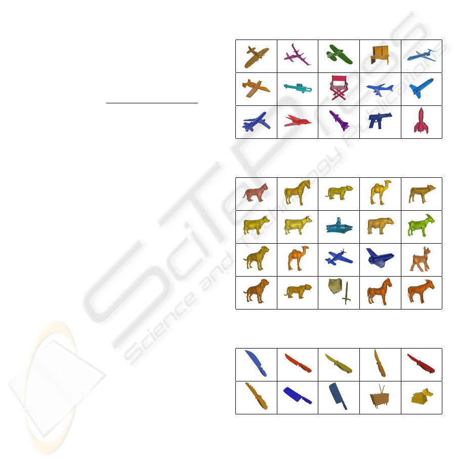
Figures 3– 6 demonstrate some of our results. In

each ﬁgure, the test object is the left-most, top ob-

ject, and the objects retrieved are ranked from left to

right. In particular, Figure 3 presents the most similar

objects to Detpl (at the top-left), as retrieved by our

algorithm. All the eight airplanes of the class were

retrieved among the top eleven. Figure 4 presents

the results of retrieving objects similar to Cat2. Six-

teen out the eighteen members of the 4-legged animal

class were retrieved among the top twenty. Figure 5

presents the retrieved most similar objects to Knifech.

Eight out of the nine knifes of the class were retrieved

among the top ten. Figure 6 demonstrates the most

similar objects to the missile at the top left, as re-

trieved by our algorithm. Six out of the the seven class

members were retrieved among the top nine. Note

that in all the above cases the members of each class

differ geometrically. Yet, their decomposition graphs

are similar and therefore they were found to be simi-

lar.

Figure 3: The most similar objects to Detpl (top left).

Figure 4: The most similar objects to Cat2.

Figure 5: The most similar objects to Knifech.

On the class of bottles, the algorithm does not per-

form as well. This class contains seven members (see

Figure 7). Though the objects seem similar geomet-

rically, their connectivity differs. The Beer, Ketchup

and Tabasco bottles consist each of 4-8 disconnected

components while Bottle3, Champagne, Whiskey and

Plastbtl consist each of only one or two components.

MESH RETRIEVAL BY COMPONENTS

147

Figure 6: The most similar objects to Aram.

Figure 7: The bottle class.

Since connectivity determines the graph structure and

the graphs differ, the results of the retrieval experi-

ments are inferior to the other classes.

All four sub-methods performed well. The Wa-

tershed decomposition performed slightly better than

convex decomposition. This fact might be surprising

since convexity is the main factor in human segmen-

tation. This can be explained by the fact that optimal

convex decomposition cannot be achieved. Moreover,

the height function used in the Watershed algorithm

considers convexity as well.

Considering only the original large components

and ignoring the small ones performs better than

merging small components with their neighbors, both

for watershed decomposition and for convex decom-

position. This can be explained by the fact that merg-

ing results in complex shapes which might cause a

failure of the basic shape determination procedure.

Table 1 shows some of our results for one sub-

method – Watershed, ignoring small components.

The ﬁrst column shows the classes and the test ob-

jects. For each class, the number of members of the

class N is shown. The next column of the table sum-

marizes the results obtained for each test object. Each

result (n/m) represents the number of the members of

the same class n retrieved among the top m objects.

6 CONCLUSION

This paper examines the adaptation of the human vi-

sion theories of Marr and Biederman to three dimen-

sions. According to these theories, an object is repre-

sented by an attributed graph, where each node repre-

sents a meaningful component of the object, and there

are arcs between nodes whose corresponding compo-

nents are adjacent in the model. Every node is at-

tributed with the basic shape found to best match the

component, while each arc is attributed with the rela-

tive surface area of its adjacent nodes.

It was demonstrated that simple and efﬁcient de-

composition algorithms sufﬁce to construct such a

Table 1: Summary of the experimental results for the Wa-

tershed / ignore sub-method.

Class(N)/

Object Retrieved / Top results

Airplanes(8)

Detplane 5/6 7/9 8/16

Worldw 6/6 6/9 8/16

747 5/6 5/9 7/16

Animals(18)

Cat2 6/8 11/14 14/20

Tiger3 7/8 11/14 13/20

Deer 8/8 11/14 15/20

Humans(19)

Woman2 10/10 17/17 19/24

Child3y 10/10 15/17 19/24

Knives(9)

Knifech 6/6 8/8 8/15

Knifest 6/6 6/8 8/15

Missiles(7)

Aram 3/6 5/10

Bottles(7)

Beer 1/3 1/6

signature. We examined a couple of post-processing

steps on top of well-known segmentation algorithms,

in order to get only a handful of components. More-

over, a technique was presented for ﬁnding the best

match between a given sub-mesh and pre-deﬁned ba-

sic shapes. An error-correcting subgraph isomor-

phism algorithm was used for matching.

The experimental results presented in the paper are

generally good. The major beneﬁts of the signature

is being invariant to non-rigid transformations and

avoiding normalization as a pre-processing step. In

addition, the algorithm for generating signatures is

simple and efﬁcient and produces very compact sig-

natures.

The technique has a couple of drawbacks. First,

the signature depends on the connectivity of the given

objects, which might cause geometrically-similar ob-

jects to be considered different. Second, the graph

matching algorithm we use is relatively slow. While

the ﬁrst drawback can be solved by ﬁxing the models,

the second problem is inherent to graph-based repre-

sentations. More efﬁcient graph matching algorithms

should be sought.

REFERENCES

Bates, D. and Watts, D. (1988). Nonlinear Regression and

Its Applications. John Wiley & Sons, New York.

Biederman, I. (1987). Recognition-by-components: A the-

ory of human image understanding. Psychological Re-

view, 94:115–147.

GRAPP 2006 - COMPUTER GRAPHICS THEORY AND APPLICATIONS

148

Biederman, I. (1988). Aspects and extensions of a theory

of human image understanding. Pylyshyn Z. editor,

Computational Processes in Human Vision: An Inter-

disciplinary Perspective, pages 370–428.

Biederman, I. (1995). Visual object recognition. S. Koss-

lyn, D. Osherson, editors. An Invitation to Cognitive

Science, 2:121–165.

Chazelle, B., Dobkin, D., Shourhura, N., and Tal, A. (1997).

Strategies for polyhedral surface decomposition: An

experimental study. Computational Geometry: The-

ory and Applications, 7(4-5):327–342.

Cornea, N., Demirci, M., Silver, D., Shokoufandeh, A.,

Dickinson, S., and Kantor, P. (2005). 3D object re-

trieval using many-to-many matching of curve skele-

tons. In IEEE International Conference on Shape

Modeling and Applications, pages 368–373.

Duda, R., Hart, P., and Stork, D. (2000). Pattern Classiﬁca-

tion. John Wiley & Sons, New York.

Elad, M., Tal, A., and Ar, S. (2001). Content based retrieval

of vrml objects - an iterative and interactive approach.

EG Multimedia, 39:97–108.

Hilaga, M., Shinagawa, Y., Kohmura, T., and Kunii, T.

(2001). Topology matching for fully automatic sim-

ilarity estimation of 3D shapes. SIGGRAPH, pages

203–212.

Katz, S., Leifman, G., and Tal, A. (2005). Mesh segmen-

tation using feature point and core extraction. The Vi-

sual Computer, 21(8-10):865–875.

Katz, S. and Tal, A. (2003). Hierarchical mesh decompo-

sition using fuzzy clustering and cuts. ACM Trans.

Graph. (SIGGRAPH), 22(3):954–961.

Kazhdan, M., Chazelle, B., Dobkin, D., and Funkhouser,

T. (2003a). A reﬂective symmetry descriptor for 3D

models. Algorithmica, page to appear.

Kazhdan, M., Funkhouser, T., and Rusinkiewicz, S.

(2003b). Rotation invariant spherical harmonic rep-

resentation of 3D shape descriptors. In Symposium on

Geometry Processing.

Keren, D., Cooper, D., and Subrahmonia., J. (1994). De-

scribing complicated objects by implicit polynomials.

IEEE Transactions on Pattern Analysis and Machine

Intelligence, 16(1):38–53.

Lee, S., Kim, J., and Groen, F. (1990). Translation-

, rotation-, and scale-invariant recognition of hand-

drawn symbols in schematic diagrams. Int. J. Pattern

Recognition and Artiﬁcial Intelligence, 4(1):1–15.

Lee, Y., Lee, S., Shamir, A., Cohen-Or, D., and Seidel, H.-

P. (2005). Mesh scissoring with minima rule and part

salience. Computer Aided Geometric Design.

Leifman, G., Meir, R., and Tal, A. (2005). Semantic-

oriented 3D shape retrieval using relevance feedback.

The Visual Computer, 21(8-10):649–658.

Li, X., Toon, T., Tan, T., and Huang, Z. (2001). Decompos-

ing polygon meshes for interactive applications. In

Proceedings of the 2001 symposium on Interactive 3D

graphics, pages 35–42.

Mangan, A. and Whitaker, R. (1999). Partitioning 3D sur-

face meshes using watershed segmentation. IEEE

Transactions on Visualization and Computer Graph-

ics, 5(4):308–321.

Marr, D. (1982). Vision - A computational investigation into

the human representation and processing of visual in-

formation. W.H. Freeman, San Francisco.

Messmer, B. (1995). GMT - Graph Matching Toolkit. PhD

thesis, University of Bern.

Osada, R., Funkhouser, T., Chazelle, B., and Dobkin, D.

(2001). Matching 3D models with shape distribu-

tions. In Proceedings of the International Conference

on Shape Modeling and Applications, pages 154–166.

Paquet, E., Murching, A., Naveen, T., Tabatabai, A., and

Rioux, M. (2000). Description of shape information

for 2-D and 3-D objects. Signal Processing: Image

Communication, pages 103–122.

Pearce, A., Caelli, T., and Bischof, W. (1994). Rulegraphs

for graph matching in pattern recognition. Pattern

Recognition, 27(9):1231–1246.

Rocha, J. and Pavlidis, T. (1994). A shape analysis model

with applications to a character recognition system.

IEEE Trans. Pattern Analysis and Machine Intelli-

gence, 16:393–404.

Shamir, A. (2004). A formalization of boundary mesh seg-

mentation. In Proceedings of the second International

Symposium on 3DPVT.

Subrahmonia, J., Cooper, D., and Keren, D. (1996). Practi-

cal reliable bayesian recognition of 2d and 3D objects

using implicit polynomials and algebraic invariants.

IEEE Transactions on Pattern Analysis and Machine

Intelligence, 18(5):7505–519.

Sundar, H., Silver, D., Gagvani, N., and Dickinson, S.

(2003). Skeleton based shape matching and retrieval.

In Shape Modelling and Applications.

Taubin, G. (1991). Estimation of planar curves, surfaces,

and nonplanar space curves deﬁned by implicit equa-

tions with applications to edge and range image seg-

mentation. IEEE Transactions on Pattern Analysis

and Machine Intelligence, 13(11):1115–1138.

Veltkamp, R. (2001). Shape matching: Similarity measures

and algorithms. In Shape Modelling International,

pages 188–197.

Vranic, D. and Saupe, D. (2002). Description of 3D-shape

using a complex function on the sphere. In Proceed-

ings IEEE International Conference on Multimedia

and Expo, pages 177–180.

Wang, Y.-K., Fan, K.-C., and Horng, J.-T. (1997). Genetic-

based search for error-correcting graph isomorphism.

IEEE Trans. Systems, Man, and Cybernetics, 27:588–

597.

Wong, E. (1992). Model matching in robot vision by sub-

graph isomorphism. Pattern Recognition, 25(3):287–

304.

Zuckerberger, E., Tal, A., and Shlafman, S. (2002). Poly-

hedral surface decomposition with applications. Com-

puters & Graphics, 26(5):733–743.

MESH RETRIEVAL BY COMPONENTS

149