
LP FITTING APPROACH FOR RECONSTRUCTING PARAMETRIC
SURFACES FROM POINTS CLOUDS
Thibault Marzais
LLAIC
IUT-D
´
epartement Informatique
63173 Aubiere Cedex
Yan Gerard, R
´
emy Malgouyres
LLAIC
IUT-D
´
epartement Informatique
63173 Aubiere Cedex
Keywords:
Surface reconstruction, Linear programming, Least Squares Fitting, B
´
ezier and B-spline surfaces.
Abstract:
We present a method to reconstruct a surface from a group of points, each provided with two parameters. The
kind of reconstructed surface can be a Bezier surface, a B-spline surface or any surface generated by a basis
of functions.
The usual method involved in such a reconstruction is the least squares approach. Our original fitting method
called LP-fitting uses a linear program for minimizing the uniform error instead of the quadratic error consid-
ered in least squares.
Experimental results comparing both approaches show that the surface obtained by LP-fitting is usually closer
(from a uniform point of view) to the initial points cloud than the surface obtained by least squares.
1 INTRODUCTION
Surface reconstruction is involved in several domains
of applications going from reverse engineering to sur-
face modeling. The problem is the computation of a
surface S passing as close as possible to each point of
a given subset of R
3
. We focus in this paper on re-
construction of parametric surfaces where F belongs
to a given linear space of functions (it is the case of
B
´
ezier and B-Spline surfaces).
The expression of the nearness between the points
cloud and the reconstructed surface requires to intro-
duce the error vector δ(S) that coordinates δ
i
(S) are
the distances between each point of index i in the in-
put and its closest point in surface S. This vector
measures the accuracy of the approximation. Thus,
the natural surface reconstruction problem is the com-
putation of a function F in the given linear space of
functions that error vector has a minimal norm (some
variants can be obtained by adding a value measuring
the smoothness of the surface, satisfaction of normal
constraints...). It is a highly non linear problem of op-
timization which has been tackled by Newton meth-
ods in (Atieg and Watson, 2004).
A more classical approach, developped in the
framework of computer graphics, consists in four con-
secutive steps. (Eck and Hoppe, 1996; Weiss et al.,
2002; Sarkar and Menq, 1991; J
¨
uttler, 1997)
1. Mesh generation from the unorganized points cloud
(α-shapes, marching cubes, Delaunay triangula-
tions) (Edelsbrunner and M
¨
ucke, 1994; Barber
et al., 1996)
2. Mesh partitionning in patches homeomorphic to
disks by using for instance tools of shape analysis.
(Eck et al., 1995)
3. Parametrization (Eck et al., 1995; Floater and Hor-
mann, 2005)
4. Surface fitting. After the parametrization step, a
pair of parameters (s
i
,t
i
) has been assigned to each
point (x
i
,y
i
,z
i
). The problem of surface fitting is
now to minimize the distances between each point
and its corresponding point of the surface F (s
i
,t
i
)
instead of minimizing its real minimal distance to
S.
The standard approach of surface fitting is to min-
imize
i
d
2
((x
i
,y
i
,z
i
),F(s
i
,t
i
))
2
(where d
2
is the
Euclidian distance) in the considered linear space of
functions. This objective function is the square of the
Euclidian norm ||δ||
2
where the coordinate δ
i
is the
Euclidian distance between the input point (x
i
,y
i
,z
i
)
and its corresponding point on the surface F (s
i
,t
i
).
325
Marzais T., Gerard Y. and Malgouyres R. (2006).
LP FITTING APPROACH FOR RECONSTRUCTING PARAMETRIC SURFACES FROM POINTS CLOUDS.
In Proceedings of the First International Conference on Computer Graphics Theory and Applications, pages 325-330
DOI: 10.5220/0001353503250330
Copyright
c
SciTePress

This usual routine of the overall reconstruction prob-
lem is called ”least-squares fitting” (Farin, 2002; Co-
hen et al., 2001) because the computation can be done
easily by the least squares method.
The task of the paper is to introduce an alterna-
tive to least-squares fitting and to compare both ap-
proaches. The main idea is to use the uniform norm
|| . ||
∞
instead of the Euclidian norm. We mini-
mize ||δ||
∞
where coordinate δ
i
is the uniform dis-
tance between the input point (x
i
,y
i
,z
i
) and its cor-
responding point in the surface F (s
i
,t
i
). More pre-
cisely we minimize independently the three infinite
norms ||(x
i
−F
x
(s
i
,t
i
))||
∞
, ||(y
i
−F
y
(s
i
,t
i
))||
∞
and
||(z
i
− F
z
(s
i
,t
i
))||
∞
. These problems of optimiza-
tion are linear and thus they can be solved by linear
programming. We call this approach ”LP-fitting”. Its
principle is to control the maximal distance between
each point of the input (x
i
,y
i
,z
i
) and its correspond-
ing point in the surface F (s
i
,t
i
) while the principle
of least squares fitting is to search the best solution
from a statistical point of view.
We start the paper with the basic definitions and no-
tations (see §2). We introduce in §3 the fitting prob-
lems obtained by using Euclidian or uniform norms
and their solutions by least-square method or linear
programming. We end the paper with the compari-
son of the experimental results provided by both ap-
proaches (see §4).
2 NOTATIONS
We begin with a brief introduction to classical para-
metric surfaces.
2.1 Parametric Surfaces
Let P
i
, i ∈ [[ 0 ,n]] be a subset of points of R
3
. Let
f
i
(s, t), i ∈ [[ 0 ,n]] be a family of functions and let the
parametric surface S be the image of interval product
[a, b] × [c, d] by function :
F (s, t)=
n
i=0
P
i
f
i
(s, t)
The points P
i
are called control points of surface
S. The most usual cases are B
´
ezier and B-Spline sur-
faces, depending on the family f
i
we choose.
2.2 B
´
ezier Surfaces
B
´
ezier surfaces are parametric polynomial surfaces
with bounded degree. Any basis of polynomials could
be used as functions f
i
(s, t) but the usual choice is to
work with Bernstein polynomials B
i,n
(t)=
n
i
∗ t
i
∗
(1 − t)
n−i
or more precisely with their tensor prod-
uct (their sum being 1, the surface belongs to the the
convex hull of the control points) :
F (s, t)=
m
i=0
n
j=0
P
i,j
B
i,m
(s)B
j,n
(t)
2.3 B-Spline Surfaces
The B-Spline surfaces require other parameters. We
introduce two integers k and l and two vectors S =
{s
0
,...,s
m+k−1
} and T = {t
0
,...,t
n+l−1
}, with
s
0
≤ s
1
≤ ... ≤ s
m+k−1
and t
0
≤ t
1
≤ ... ≤
t
n+l−1
called knot vectors. Then the considered fam-
ily of functions is obtained with tensor product :
F (s, t)=
m
i=0
n
j=0
P
i,j
N
i,k
(s)N
j,l
(t)
where the N
i,k
is the basis function defined by Cox
de Boor formula (Farin, 2002).
Note that by adjusting the number of parameters
by tensor product and by changing the dimension by
cartesian product, previous definitions and next re-
sults hold in a general framework.
3 SURFACE RECONSTRUCTION
3.1 General Problem
Let {M
k
}
1≤k≤p
, with M
k
=(
x
k
,y
k
,z
k
)
T
,be
a subset of p points in R
3
. We consider that each point
M
k
is provided in the input with a pair of parameters
s
k
and t
k
. The purpose of this section is to find a para-
metric surface S, defined by a function F (s, t), which
is close (in a sense to be defined) to the given set of
points. We introduce the error δ
k
of the approxima-
tion on the point M
k
:
δ
k
= F (s
k
,t
k
) − M
k
for 1 ≤ k ≤ p (1)
with a function F chosen in the linear space gener-
ated by functions (f
i
)
0≤i≤n
defined in Section 2.1.
3.2 Interpolation
If the error is constrained to be null, equalities δ
k
=0
for k ∈ [[ 1 ,p]] leads to the linear system of equations
M
k
=
n
i=0
P
i
f
i
(s, t) that unknowns are the three
coordinates of each control point P
x
i
, P
y
i
and P
z
i
.
We can be sure of the existence of a solution if the
dimension of the basis of functions f
i
is at least equal
to the number of points p. Otherwise, the linear sys-
tem is much often not feasible with the consequence
GRAPP 2006 - COMPUTER GRAPHICS THEORY AND APPLICATIONS
326
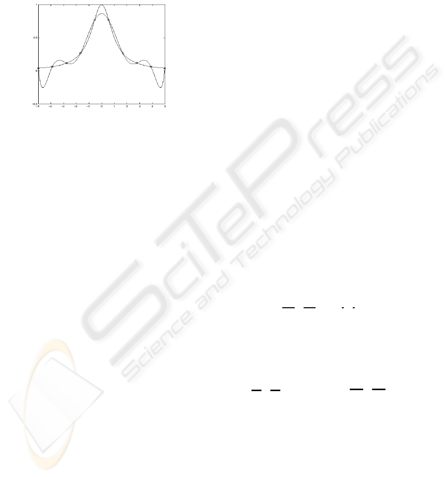
that usually no interpolation exists. This usual case
is the framework of fitting methods. Their task is to
find approximate solutions of unfeasible systems. It
allows to work with linear spaces of restricted dimen-
sions while the huge dimensions and degrees neces-
sary for interpolation introduce detrimental variations
(Figure 1).
Figure 1: Consequences of interpolation with a high degree
polynomial.
3.3 Approximate Reconstruction
The function F (s, t) of the linear space
generated by functions f
i
is denoted
F (s, t)=(x(s, t),y(s, t),z(s, t)) with
⎧
⎨
⎩
x(s, t)=
n
i=0
P
x
i
∗ f
i
(s, t)
y(s, t)=
n
i=0
P
y
i
∗ f
i
(s, t)
z(s, t)=
n
i=0
P
z
i
∗ f
i
(s, t)
and where
P
i
=
P
x
i
,P
y
i
,P
z
i
T
, i ∈ [[ 0 ,n]] are the
control points of surface F .
The principle of fitting methods is to minimize the
error expressed by Equation 1:
⎧
⎪
⎨
⎪
⎩
δ
x
k
=
n
i=0
P
x
i
∗ f
i
(s
k
,t
k
) − x
k
∀k ∈ [[ 1 ,p]]
δ
y
k
=
n
i=0
P
y
i
∗ f
i
(s
k
,t
k
) − y
k
∀k ∈ [[ 1 ,p]]
δ
z
k
=
n
i=0
P
z
i
∗ f
i
(s
k
,t
k
) − z
k
∀k ∈ [[ 1 ,p]]
Let us note that the three systems are independent
(their unknowns are different). Equation on the x-
coordinates leads to system 2 :
A ∗ X = Y + δ (2)
where A is matrix
⎛
⎜
⎜
⎝
f
0
(s
1
,t
1
) ... f
n
(s
1
,t
1
)
f
0
(s
2
,t
2
) f
n
(s
2
,t
2
)
.
.
.
.
.
.
f
0
(s
p
,t
p
) ... f
n
(s
p
,t
p
)
⎞
⎟
⎟
⎠
where vector X =(
P
x
0
, ..., P
x
n
)
T
con-
tains the x-coordinates of the control points, Y =
(
x
1
, ..., x
p
)
T
contains the x-coordinates of
the real points, and δ =
δ
x
1
, ..., δ
x
p
T
is the
error on the x-coordinates.
In the framework of interpolation, δ is constrained
to be null but we have seen in previous section that in
many cases, the linear rank of matrix A is not suffi-
cient to guarantee the existence of an exact solution.
Thus the idea of fitting methods is to optimize the vec-
tor δ according to some criteria.
3.4 Least Squares Fitting
The criteria of least squares fitting is the Euclidian
norm of the error δ
2
(Cohen et al., 2001; Farin,
2002). Equation 2 leads to the following problem of
minimization:
Min
X
A ∗ X − Y
2
⇐⇒
⎧
⎪
⎪
⎪
⎨
⎪
⎪
⎪
⎩
Min
X
p
i=1
δ
i
2
δ = A ∗ X − Y =
⎛
⎜
⎝
δ
1
.
.
.
δ
p
⎞
⎟
⎠
Thus the problem is to minimize the distance be-
tween the given point Y and a point A ∗ X belonging
to linear space Im(A). It is well known (Whittaker
and Robinson, 1967) that the the minimum is ob-
tained with the orthogonal projection of Y on Im(A)
namely with Y = A ∗ X + δ and δ ∈ Im(A)
⊥
.
This decomposition of Y (corresponding to the di-
rect sum R
p
= Im(A) ⊕ Im(A)
⊥
) is denoted :
A ∗ X
LSF
∈Im(A)
− δ
LSF
∈Im(A)
⊥
= Y
By recalling that Im(A)
⊥
is also KerA
T
,we
have :
(A
T
∗ A)
square matrix, symmetric
∗X
LSF
− A
T
∗ δ
LSF
=0
= A
T
∗ Y
and by multiplying on the left by the inverse of
A ∗ A
T
(we assume that A is a full rank matrix), it
provides the following expression of the least squares
solution :
X
LSF
=(A
T
∗ A)
−1
∗ A
T
∗ Y (3)
The n+1coordinates of X
LSF
are the coordinates
(in present case : the x-coordinates) of the n +1con-
trol points of the least squares fitting reconstructed
surface.
LP FITTING APPROACH FOR RECONSTRUCTING PARAMETRIC SURFACES FROM POINTS CLOUDS
327
3.5 LP Fitting
Our original approach consists in working with a uni-
form criterion on the error. We minimize the uniform
norm of δ instead of the Euclidian norm used in least
squares fitting. This method leads us to a linear pro-
gram (Chvatal and Vasek, 1983). According to Equa-
tion 2 we obtain the following problem of minimiza-
tion :
Min
X
A ∗ X − Y
∞
⇐⇒
⎧
⎪
⎪
⎪
⎪
⎪
⎨
⎪
⎪
⎪
⎪
⎪
⎩
Min
X
Max
1≤i≤p
|δ
i
|
δ = A ∗ X − Y =
⎛
⎜
⎝
δ
1
.
.
.
δ
p
⎞
⎟
⎠
The problem can be modified by introducing an
auxiliary real variable that we denote h. It plays the
role of a bound on the each coordinate of A ∗ X − Y .
⎧
⎨
⎩
Min
X
Max
1≤i≤p
|δ
i
|
δ = A ∗ X − Y
⇐⇒
⎧
⎨
⎩
Min
X,h
(h)
δ = A ∗ X − Y
−h ≤ δ
i
≤ +h ∀i, 1 ≤ i ≤ p
⇐⇒
Min
X,h
(h)
−h ∗ 1l ≤ A ∗ X − Y ≤ h ∗ 1l
⇐⇒
⎧
⎨
⎩
Min
X,h
(h)
A ∗ X + h ∗ 1l ≥ Y
A ∗ X − h ∗ 1l ≤ Y
It leads to the following linear program 4:
⎧
⎪
⎪
⎪
⎪
⎪
⎪
⎪
⎪
⎪
⎪
⎨
⎪
⎪
⎪
⎪
⎪
⎪
⎪
⎪
⎪
⎪
⎩
Min
X
(h)
⎛
⎜
⎝
1
A
.
.
.
1
⎞
⎟
⎠
∗
X
h
≥ Y
⎛
⎜
⎝
−1
A
.
.
.
−1
⎞
⎟
⎠
∗
X
h
≤ Y
(4)
where the variables are X ∈ R
n+1
(or each co-
ordinate of X) and h ∈ R and where the objective
function is the linear form h. By construction, the lin-
ear program is feasible. Its solution is denoted X
LP F
.
Its n +1coordinates are again the coordinates (in our
case the x-coordinates) of the n +1control points of
the LP-fitting reconstructed surface.
4 RESULTS
4.1 Protocole
We have generated point clouds from existing para-
metric surfaces: B
´
ezier surfaces, B-spline surfaces
and sphere surfaces with spherical angles as parame-
ters. The coordinates of the points and the corre-
sponding parameters have been perturbed by gaussian
noise to obtain relatively realistic points clouds. Then
we proceeded with the reconstruction according to
least squares and LP fitting methods. The results have
been recorded in histograms in order to understand
the relative merit of our new fitting method with re-
spect to classical least squares approach.
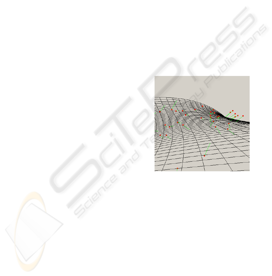
4.2 Interpretation of Results
For each surface that we reconstructed, we computed
the errors on each point (see Figure 2) .
Figure 2: Result of reconstruction with the original 3D co-
ordinates M
k
in red, the surface F (s, t) in black, and the
error vectors δ
k
=
−−−−−−−−→
M
k
F (s
k
,t
k
) in green.
Figures 3 and 4 show the reconstruction of the
same perturbed sphere by B
´
ezier surface, with the two
methods. We can notice that the least squares fitting
result seems to be a practically perfect sphere while
the LP fitting result is bumpy. It is the consequence of
an expectable behavior. The noise that we have intro-
duced on the sphere has a deeper impact on the LP-
approach than on least squares fitting. This feature
of both methods is a great difference. Least squares
would be better to deal with noisy data but there is
the risk that some important details represented only
by few points or a lower density of points in the input
could be treated as noise and disappear from the re-
constructed surface. With least squares fitting, the re-
constructed surface could be very far from one point
because the quadratic criteria has favored a solution
GRAPP 2006 - COMPUTER GRAPHICS THEORY AND APPLICATIONS
328
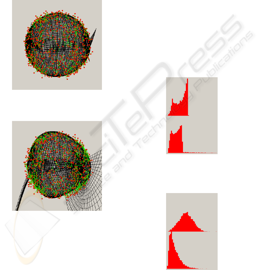
passing close to another region with a lot of points.
With LP-fitting, the uniform criterion constrains the
solution to be close to any point without any consider-
ation on its statistical weight. Thus LP-fitting is better
if all the points have an equivalent signification and
is probably less satisfying than least squares fitting if
the input is noisy (with non significant points in the
input).
Figure 3: Reconstruction of sphere with Least Squares Fit-
ting (LSF).
Figure 4: Reconstruction of sphere with LP Fitting (LPF).
4.3 Histograms
For each reconstructed surface, the Euclidian norms
of the error vectors (in green in the figures) have been
recorded in histograms.
In most cases the maximal error between a point
and its corresponding point belonging to the recon-
structed surface is much smaller with LP-fitting than
with least squares fitting (see for instance Figure 5).
There exist actualy some cases where the tendency is
inverted (see Figure 6). It is due to the fact that the
maximum of the error on the x-coordinate, on the y-
coordinate and on the z-coordinate are obtained with
points of different indices with the consequence that
an independent minimization of each of them (what is
done in LP-fitting) does not guarantee to minimize the
maximum of their Euclidian norm. Some more stan-
dard histograms are drawn in Figure 7 and 8. They
show results with little disturbed data and much more
disturbed data. In general, on all computed examples,
with few and much more disturbances, the LP-fitting
maximum error is about 80% of the least squares
maximum error.
The main result of our experiment is that LP-fitting
provides surfaces which are significantly closer from
the points cloud in terms of maximal distance. We
can also notice on the shape of the corresponding his-
tograms that by using LP-fitting the cost on the mean
error (which is minimum by using least squares fit-
ting) remains quite low.
Figure 5: Histograms of reconstruction of a perturbed
sphere by B
´
ezier surface 5*5 : LP-fitting (top) least squares
fitting (bottom).
Figure 6: Histograms of reconstruction of another perturbed
sphere by B
´
ezier 5*5 : LP-fitting (top) least squares fitting
(bottom).
LP FITTING APPROACH FOR RECONSTRUCTING PARAMETRIC SURFACES FROM POINTS CLOUDS
329
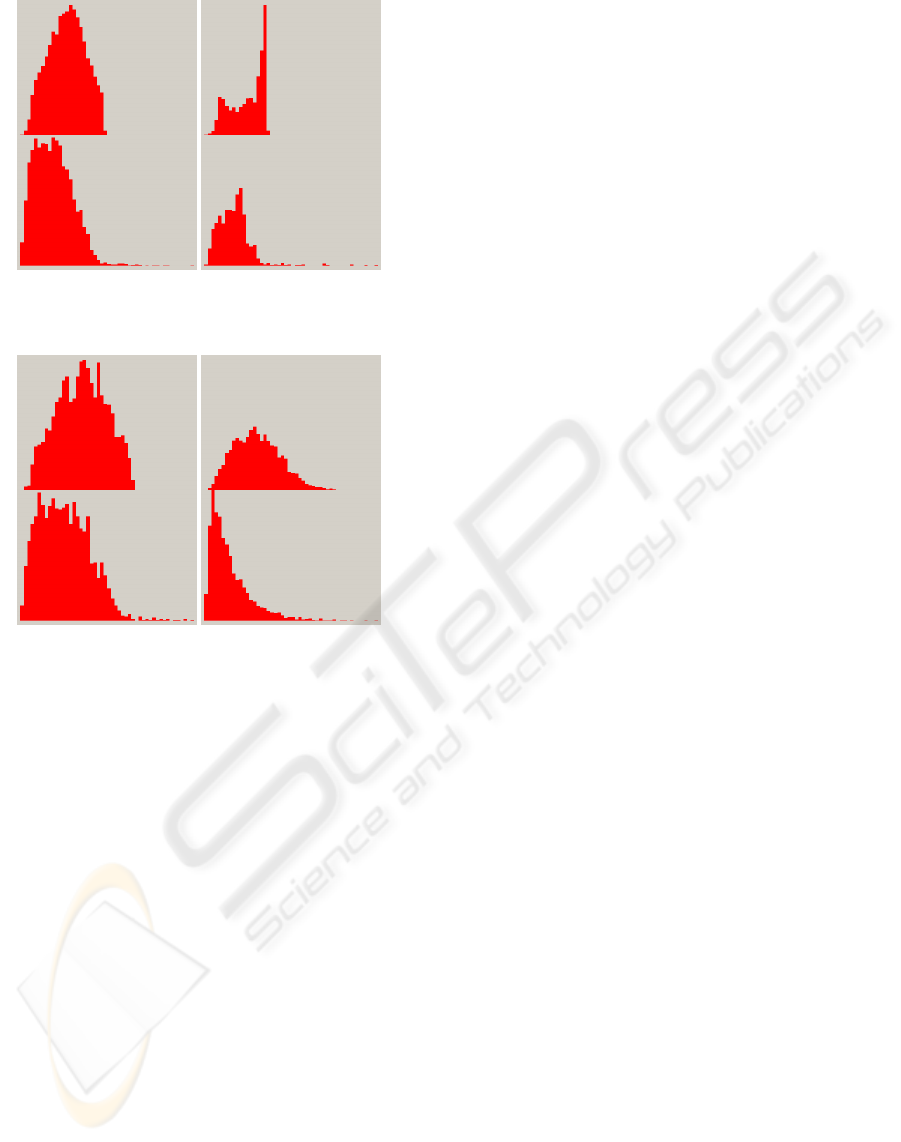
Figure 7: Two histograms of reconstructions : LP-fitting
(top) least squares fitting (bottom).
Figure 8: Two histograms of reconstructions of highly per-
turbed input : LP-fitting (top) least squares fitting (bottom).
5 CONCLUSION
Least squares fitting is a subroutine of the general
problem of surface reconstruction. The input is a fi-
nite subset of R
3
provided with a pair of parameters
for each point. The output is a grid of control points
ofaB
´
ezier, B-spline surface (or any surface of the
same kind). We propose in this paper an alternative
method based on the idea to minimize the uniform er-
ror on the input instead of usual quadratic Euclidian
error. From a computational point of view, it leads
to a linear program which can be solved by any solver
while classical least squares approach only requires to
compute an orthogonal projection on a linear space.
The different features of the two methods are re-
lated to the choice to minimize the uniform or Euclid-
ian error. With least squares approach the statistical
weight of a subset of points concentrated in a given
region enforces the reconstructed surface to be close
to it while an isolated point can be considered as noise
with the consequence that the surface can be far from
it. With LP-fitting the reconstructed surface is close
to all the points of the input independently of their
number in each region. This different behavior is the
main point allowing to choose one or the other fitting
method.
REFERENCES
Atieg, A. and Watson, G. A. (2004). Use of l
p
norms in
fitting curves and surfaces to data. In Crawford, J. and
Roberts, A. J., editors, Proc. of 11th Computational
Techniques and Applications Conference CTAC-2003,
volume 45, pages C187–C200.
Barber, C. B., Dobkin, D. P., and Huhdanpaa, H. (1996).
The quickhull algorithm for convex hulls. ACM Trans-
actions on Mathematical Software, 22(4):469–483.
Chvatal and Vasek (1983). Linear Programming. A Series
of Books in the Mathematical Sciences. W. H. Free-
man and Company, New York.
Cohen, E., Riesenfield, R. F., and Elber, G. (2001). Geo-
metric Modeling with Splines : An Introduction.AK
Peters.
Eck, M., DeRose, T., Duchamp, T., Hoppe, H., Lounsbery,
M., and Stuetzle, W. (1995). Multiresolution analysis
of arbitrary meshes. Computer Graphics, 29(Annual
Conference Series):173–182.
Eck, M. and Hoppe, H. (1996). Automatic reconstruction
of B-Spline surfaces of arbitrary topological type. In
ACM SIGGRAPH 96, pages 325–334.
Edelsbrunner, H. and M
¨
ucke, E. P. (1994). Three-
dimensional alpha shapes. ACM Transactions on
Graphics, 13(1):43–72.
Farin, G. (2002). Curves and surfaces for CAGD: a practi-
cal guide. Morgan Kaufmann Publishers Inc.
Floater, M. S. and Hormann, K. (2005). Surface parame-
terization: a tutorial and survey. In Dodgson, N. A.,
Floater, M. S., and Sabin, M. A., editors, Advances in
multiresolution for geometric modelling, pages 157–
186. Springer Verlag.
J
¨
uttler, B. (1997). Surface fitting using convex tensor-
product splines. J. Comput. Appl. Math., 84(1):23–44.
Sarkar, B. and Menq, C.-H. (1991). Smooth-surface ap-
proximation and reverse engineering. Computer-
Aided Design, 23(9):623–628.
Weiss, V., Andor, L., Renner, G., and V
´
arady, T. (2002).
Advanced surface fitting techniques. Comput. Aided
Geom. Des., 19(1):19–42.
Whittaker, E. T. and Robinson, G. (1967). The Method of
Least Squares. Ch. 9 in The Calculus of Observations:
A Treatise on Numerical Mathematics. Dover Publi-
cations, 4th edition.
GRAPP 2006 - COMPUTER GRAPHICS THEORY AND APPLICATIONS
330
