
INTERACTION BETWEEN WATER AND
DYNAMIC SOFT BODIES
Tatiana Alexandrova, Olivier Terraz, Djamchid Ghazanfarpour
XLIM Laboratory UMR CNRS 6172, University of Limoges,83 rue d’Isle,87000 Limoges, France
Keywords: liquid animation, movement simulation, dynamic soft body, Lattice-Boltzmann method.
Abstract: The water animation by moving soft bodies, changing their shapes, is the subject of the present work. The
mechanism of movement transformation from a body to a liquid is elaborated on the basis of Lattice-
Boltzmann method of fluid modeling. The use of boundary conditions, destined to perform this
transformation visually realistic and computationally quite inexpensive, is one of the main innovations of
our approach. The model is applied to the jellyfish propulsion water.
1 INTRODUCTION
The subject of this work is a physically based
modeling of a liquid animation caused by a soft
dynamic body movement. In computer graphics,
physical based models have an important advantage
compared to empiric ones. They make the scene
evolve automatically and do not require the user
intervention for each animation step. Once the
relations and laws of interaction among objects
and/or medium are given, the correctly produced
system automatically simulates the behavior of the
whole scene. This gives essential increasing of
computational time. Recent physically based models
(Guendelman, Selle, Losasso, Fedkiw, 2005),
(Muller, Solenthaler, Keiser, Gross, 2005) are
developed in order to maximally reduce the
calculation time and to present visual plausibility,
keeping the details of a real world animation.
The model presented in this paper proposes a
quite simple way of transforming body motion to
liquid motion. The special, easy to apply boundary
conditions are elaborated in application to the
Lattice Boltzmann method for this purpose. The
model is applied to underwater scenes with
swimming jellyfish. The simulations of jellyfish
movement and its interaction with particles in water
and with algae are performed.
The paper is composed as follows. In the second
part, the liquid animation models are discussed. The
third part is devoted to the transformation of soft
body movement to surrounding water and
consequently to neighboring objects. In this part, we
can find the main innovation of this work: the
boundary conditions for moving soft bodies. The
fourth part presents the results obtained by this
method. The last section concerns conclusions and
future work.
2 ANIMATION OF LIQUIDS
In this section we give a brief review of liquid
modeling. There are the fluid dynamics methods,
simplified to satisfy the needs of computer graphics.
Computational fluid dynamics proposes a variety
of tools for fluid motion modeling, but it demands
special skills and resists external control. In addition,
it is very time consuming. In order to be applied in
computer graphics, simplified physically based
approaches were intensively developed during recent
years. To introduce first branch, one can refer to
(Foster, Metaxas, 1996), (Stam, 1999), (Foster,
Fedkiw, R., 2001). Visual fidelity is the main goal of
these models. These methods solve the Navier-
Stokes equations on a discrete voxel grid that causes
decreasing the time step or refinement of a grid
when the boundary geometry is complex.
There are several problems already considered in
this branch of liquid modeling; the models were
essentially improved compared to the first ones. In
(Genevaux, Habibi, Dischler, 2003) the fluid-solid
interaction was explored; the method is based
mainly on the definition of a coupling force between
384
Alexandrova T., Terraz O. and Ghazanfarpour D. (2006).
INTERACTION BETWEEN WATER AND DYNAMIC SOFT BODIES.
In Proceedings of the First International Conference on Computer Graphics Theory and Applications, pages 384-391
DOI: 10.5220/0001357003840391
Copyright
c
SciTePress
the solids and the fluid. In (Guendelman, Selle,
Losasso, Fedkiw, 2005) the method for water - cloth
interaction, well suiting also to water - air and solid -
fluid interface, is given. The rigid body - fluid
interplay is presented by a Rigid-Fluid method in
(Carlson, Mucha, Turk, 2004).
Recently, the Smoothed Particle Hydrodynamics
method was presented in application to fluid - fluid
interaction, water pouring into a glass and
interaction of fluid with deformable solids (Muller,
Solenthaler, Keiser, Gross, 2005), (Muller,
Charypar, Gross, 2003), (Muller, Schrim, Teschner,
Heidelberger, Gross, 2004).
The other direction in flow simulation is the
Lattice-Boltzmann method (LBM) (Chen, Doolean,
1998), (Wei Li, Zhe Fan, Xiaoming Wei, Arie
Kaufman, 2003). It gives a microscopic
representation of a fluid as a set of microscopic
particles. The method is derived from the Boltzmann
equation from the kinetic theory of gases. Almost all
Lattice-Boltzmann equations simulate compressible
fluids with some finite sound speed c
s
. However the
computed solutions are expected to converge to
incompressible limit, when the liquid speed |
u
ρ
| is
sufficiently small compared to the sound speed c
s
(Mach number
0/ →=
sa
cuM
ρ
).
Let us consider the principles of LBM. The
liquid is represented by a finite regular grid and by a
set of a packet distribution values
{
}
qi
f for each cell
of a grid. Each packet distribution value
qi
f
corresponds to the velocity direction vector
qi
e
ρ
shooting from a node to its neighbor. A pair
(
qi
f ,
qi
e
ρ
) indicates how many particles
qi
f in the
cell have the velocity direction
qi
e
ρ
.
It is supposed that there always exists a local
equilibrium particle distribution
eq
qi
f dependent only
on the density
ρ
, and on the local fluid velocity
ν
ρ
.
The LBM updates the packet distribution values at
each cell based on two rules:
collision:
qiqi
new
qi
tXftXf Ω=− ),(),(
(1)
propagation:
),()1,( tXfteXf
new
qiqiqi
=++
ρ
(2)
where X is the coordinate in R
3
, and
qi
Ω is the
general collision operator. Since the components of
qi
e
ρ
can only be chosen from {-1, 0, 1}, the
propagation is local.
Collision describes the redistribution of packets
at each local node. Propagation means the packet
distributions move to the nearest neighbor along the
velocity direction.
The density and velocity are calculated for each
cell from the packet distributions as follows (
Wei Li,
Zhe Fan, Xiaoming Wei, Arie Kaufman, 2003):
∑
=
qi
qi
f
ρ
,
qi
qi
qi
ef
ρ
ρ
∑
=
ρ
ν
1
.
Mass and momentum are conserved locally.
Then, the collision step (with commonly used BGK
collision term (Bhatnagar, Gross, Krook, 1954)) is:
()
),(),(
1
),(),( vftXftXfvf
eq
qiqiqi
new
qi
ρ
τ
ρ
−−=−
,
where τ is a relaxation time (timescale for which
every variable relaxes towards equilibrium), which
determines the viscosity of the flow,
eq
qi
f
is the
local equilibrium distribution function.
A great advantage of this method is that it
supports dynamic boundary conditions. For more
details see (Chen, Doolean, 1998), (Wei Li, Zhe Fan,
Xiaoming Wei, Arie Kaufman, 2003).
There exist the following usual models with a
rest particle for 3D space (see Fig.1): D3Q15 (fifteen
velocities), D3Q19 (nineteen velocities), D3Q27
(twenty seven velocities) (Renwei Mei, Wei Shyy,
Dazhi Yu, Li-Shi Luo, 2002). A minor variation of
those models is to remove the rest particles from the
discrete velocity set; the resulting models are known
as the D3Q14, D3Q18, and D3Q26 models,
respectively. The LBM with a rest particle generally
have better computational stability.
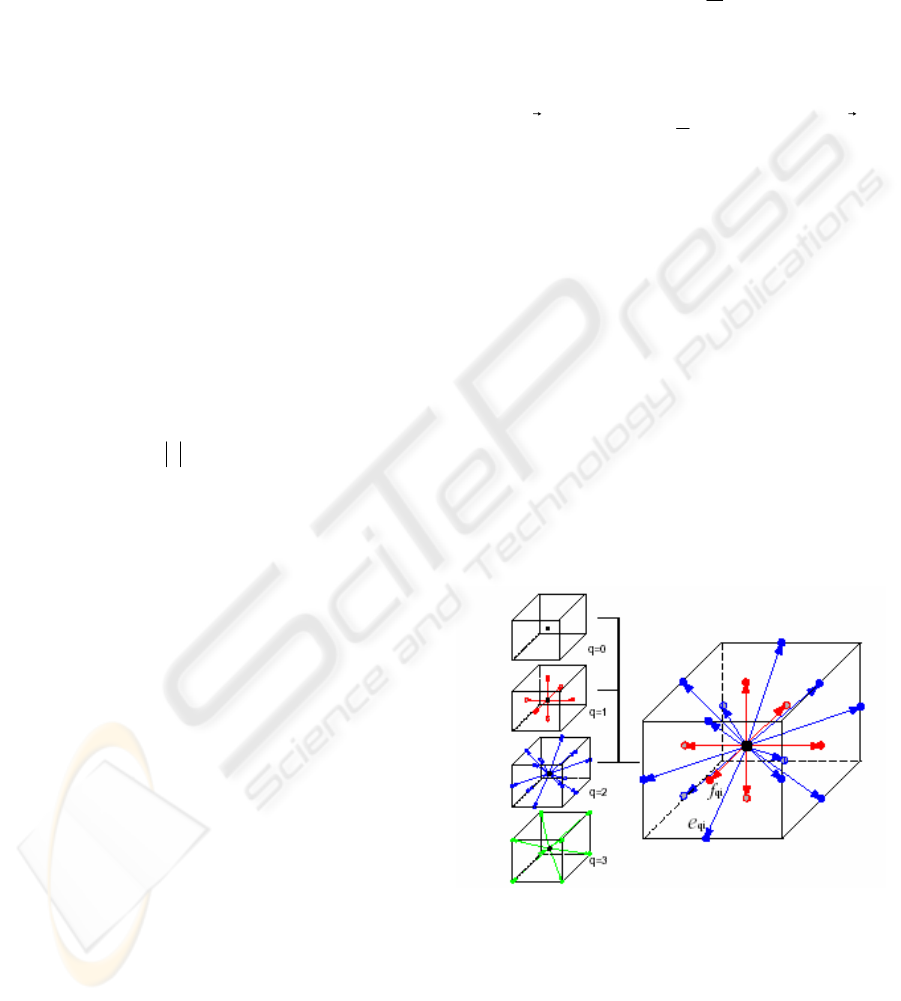
Figure 1: 3D lattice geometry. On the left side there are
presented the four sub-lattices that are defined in a 3D
lattice. On the right side is the combination of sub-lattices
0, 1, and 2 (19 packets) (Wei Li, Zhe Fan, Xiaoming Wei,
Arie Kaufman, 2003).
In the present work the D3Q15 model is taken,
the simplest model for 3D space, in our case it suits
well due to the smoothness of the movement and the
simplicity of the scene objects:
INTERACTION BETWEEN WATER AND DYNAMIC SOFT BODIES
385
⎪
⎪
⎩
⎪
⎪
⎨
⎧
=±±±
=±±±
=
=
IIgroupi
Igroupi
particleresti
e
i
14,...,7)1,1,1(
6,...,1)1,0,0(),0,1,0(),0,0,1(
,0)0,0,0(
3 TRANSFORMATION OF BODY
MOVEMENT TO A LIQUID
MOVEMENT
The movement of the dynamic body, once properly
transferred, animates the liquid and neighboring soft
bodies, the passive and the active ones. An example
is the swimming jellyfish, which can transfer the
motion to other jellyfishes and algae surrounding it.
Let us suppose that the parameters of dynamic
body surface, such as coordinates and velocities of
the control points, are known at each time step. The
most important part in a water animation by a body
is the interaction, where the movement of a dynamic
surface should be properly transferred to the lattice
cells. Here we are restricted to one-way
transformation of movement, which means that the
body is not influenced by a liquid but acts as a motor
of a motion. The full interaction, the reciprocal
influence of the body and the liquid complicates the
problem.
The transformation of the movement is done
with assigning local surface velocities to the
boundary lattice cells touching the jellyfish surface
and their subsequent influence on the other cells. At
the starting point at time
0=t
the uniform
equilibrium distribution with velocity
0
=
u
and
constant water density is assigned to all lattice cells.
The coordinate of a unit cell is a vector, formed
by the minimal integer numbers of cell points
coordinates. So, the point (-5.3, 2.6, 0.1) belongs to
the cell with coordinates (-6, 2, 0).
Further, we consider the swimming jellyfish as
an example. The movement of the jellyfish suits to
our aim of deforming body – liquid interaction
simulation. The movement consists of contraction
and relaxation of the bell forming the body, so the
jellyfish opens and closes its bell.
Now we have to explain briefly the model of
jellyfish body and its animation model made here.
The jellyfish is presented as a NURBS surface with
axial symmetry (see Fig. 2). For the deformation a
dynamic particle system is used; the particles are
shown in the figure with points. The particle system
is a set of unit-masses, where the forces are applied.
The particles are placed in 96 CVs, the control
points, which control the shape of the surface.
For a better implementation of the deformation
system in the present model, the particles were
placed in CVs and then the shape of the surface was
modified. Particles positions at the low part of
jellyfish do not correspond to CV positions, but still
keep connection; the particle translations are applied
to corresponding CVs.
Jellyfish contractions are simulated by 10
axisymmetric mass-spring systems. Each spring acts
accordingly to its rigidity, a length at rest, and
weights of the particles at the ends. At the beginning
the springs are supposed to be stretched, that gives a
contraction. At the relaxation phase, the springs are
supposed to be compressed. For simplicity, the
properties of the springs are changed at certain time
points during scene evaluation in order to alternate
contractions and relaxations.
Figure 2: Jellyfish model with particle system and mass-
spring system.
As we know the coordinates of the control points
of the body, these 3D coordinates determine the
corresponding boundary cells; the velocities of the
control points allow the calculation of the packet
distributions for LBM. They can be taken as the
equilibrium distributions with the local surface
velocity and a constant water density for all cells, as
the water is a non-compressible liquid. Linear
interpolation is applied to calculate coordinates and
velocities of the cells in between the control points.
The lattice is finite and the boundary conditions
are to be set for the boundaries of the lattice, as well
as for the boundaries of the body.
3.1 Boundary Conditions on the
Lattice Border
Boundary conditions in the LBM may take several
forms (Wei Li, Zhe Fan, Xiaoming Wei, Arie
Kaufman, 2003). The conditions that can be applied
to the border of the lattice include periodic boundary
GRAPP 2006 - COMPUTER GRAPHICS THEORY AND APPLICATIONS
386
and outflow boundary. For periodic boundary, the
outgoing distributions wrap around and re-enter the
lattice from the other side. For outflow boundary,
distributions propagating outside the lattice are
simply discarded. However, boundary cells also
have some distributions propagating inwards from
fictitious cells just outside the boundary.
3.2 Boundary Conditions on the
Body
Now let us consider obstacle boundaries, which
should be set for objects inside the lattice. The “no-
slip” boundary condition requires that the tangential
component of the fluid velocity along the boundary
be zero. The simple implementation is a bounce-
back rule. The outgoing distribution, facing the
boundary, re-enters the lattice at the same cell, but
associated with the opposite velocity.
In (Wei Li, Zhe Fan, Xiaoming Wei, Arie
Kaufman, 2003) improved boundary conditions are
applied to complex geometries and moving
boundaries. They are represented as a complex
function including neighbor cell distributions,
velocity of the local surface, proportional distances
to the cell nodes (coordinate points) and surrounding
water velocities.
In the present work the moving boundaries are
treated in different manner. The main purpose of
proposed boundaries is to transfer the movement
from object to water independently of surrounding
water velocities. This is the main distinction of our
method. The boundary cells are, in some way, the
fictitious cells. They affect the other lattice cells, but
are not affected by other cells. The properties of
these cells depend totally on the local surface
velocity. The velocity distributions in these cells are
set to the equilibrium values. The aim is to transfer
the object-in-water motion properly and in a simple
manner. The method proposed, uses the bounce-
back rule in combination with the interaction with
the fictitious boundary cells.
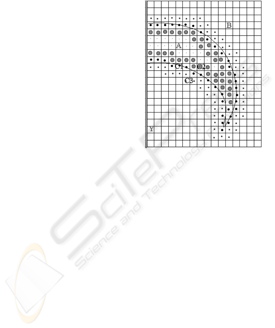
The lattice cells are separated in three groups,
see Fig.3. The first one (group A) is the group of
body inner cells. Inner cells mean the cells, which
stay inside the body as well as all of its neighbors.
These cells are passive and the distributions for them
are not calculated, they keep zero.
The second group (group B) includes water cells.
These are the cells, which are the cells of water as
well as all of its neighbors. The velocities of these
cells are calculated according to the standard
procedure in two steps: collision and streaming.
The third group (group C) is the boundary and
pre-boundary cells. This group is the most important
and is again divided into three groups:
Figure 3: Groups of lattice cells: A are the inner cells, B
are the water cells, C1, C2, C3 are the boundary cells.
1. boundary cells (group C1)
2. inner cells of the body which have at least
one boundary cell as a neighbor (group C2)
3. water cells which have at least one
boundary cell as a neighbor (group C3).
Further, we will discuss group C and its under-
groups. The cells of the first group, C1, get the
distributions
),(
loc
eq
qi
f
νρ
ρ
depending on local surface
velocity. The remaining two groups are responsible
for proper transferring of the movement.
Let us consider group C2, the inner cells. Since
we use linear interpolation to find the water cells
intersecting with body surface in between the control
points of dynamic system, it is important to find all
the cells having exchanges with the outside cells.
They are all inner cells having, at least, one C1
neighbor. In the present model their distributions are
set as average distributions of surrounding boundary
cells C1 (inner cells A are not taken into account).
The pre-boundary cells of group C3 get the
incoming distributions from C1 and C2 at a collision
step. But their own distributions, in directions to
boundary cells C1, change the direction for opposite
and re-enter to the cell. So, at the streaming step the
pre-boundary cells C3 get the incoming distributions
from the water cells B, from boundary cells C1, C2,
and, in addition, some of their own distributions are
INTERACTION BETWEEN WATER AND DYNAMIC SOFT BODIES
387

returned as they meet a wall (body surface). During
the evaluation of the dynamic system the lattice cells
change the status and pass from one group to
another.
The time step and the lattice size should be
properly chosen because the system can become
unstable. In the LBM the indication of instability of
a solution is the appearance of negative values of
equilibrium distributions at the collision step.
Physically, the model described above is not
accurate because mass is not strictly conserved. On
the other hand, the deviation is little and the method
is simple. The important feature of Lattice-
Boltzmann Method, the support of moving
boundaries, is used here and the movement issuing
from the object is successfully transferred to the
water space.
3.3 Jellyfish Propagation in a Water
Space
One more advantage can be gained from the
proposed application of the Lattice-Boltzmann
Model, the body propagation in liquid. Having
known the velocities of boundary cells, we know,
roughly speaking, the forces with which the body
acts on the liquid in these cells.
The propagation can be calculated based on the
momentum conservation law at the interaction of
two bodies having masses m
1
, m
2
and velocities v
1
,
v
2
correspondingly, m
1
v
1
=m
2
v
2
.
In the case of a jellyfish swimming, a strong
simplification can be done. According to a
biological model, the jellyfish propagation is
generated by a cylindrical jet of water from the bell
cavity. Approximately, one can consider the two-
object system: the jellyfish and the cavity water; see
Fig.4.
Water
Jellyfish
Figure 4: Two-object system: the jellyfish and the bell
cavity water.
Here it does not matter what to consider, masses
or volumes, as the water and jellyfish densities are
almost equal. We know the volume of pushed water,
at each step it can be approximated as a sum over
boundary cells C1:
,
2
1
2
tlvV
cell
i
i
∆=∆
∑
here v
i
is the cell velocity, l
cell
is the cell size, ∆t is
the time step. Having this change of volume, we can
calculate the height of a column of water pushed by
jellyfish. The base of the column is taken as a circle
with the jellyfish aperture radius R
a
. The height of
the column is
,
2
a
R
V
h
π
∆
=
the velocity of the cavity
water is approximately taken as
t
h
v
w
∆
≈
. Now the
movement conservation law is used. Considering the
volumes in place of masses,
j
w
wj
V
V
vv =
is the
jellyfish velocity at the current step, where
3
3
4
2
1
RaV
w
π
⋅=
is the approximate cavity water
volume, and the jellyfish volume V
j
is approximately
a sum of all inner cells (group A + group C2). The
jellyfish transition is calculated as
tvl
j
∆=∆ .
This model is non-correctly physically based
during jellyfish opening, but gives visually pleasing
results.
4 RESULTS
In this section we present the results of our model
application to underwater virtual words. Scenes are
modeled in Maya 6.0. A plug-in calculating the
velocity field in water, generated by a jellyfish
swimming is written in Maya API.
Let us consider the general parameters of the
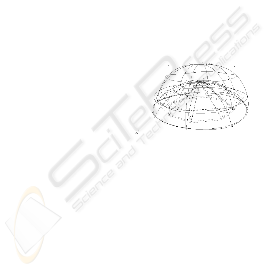
scenes. In Fig.5 the jellyfish, the dynamic body, is
presented in the scene and the size of the lattice is
shown. The jellyfish is oriented normally to the
ground, but the orientation axis can be chosen
differently. It also can be changed during the
animation simulation as a function of some factor(s).
The bell diameter of relaxed jellyfish is about 40 cm,
and the field lattice cube size is 80 cm. In the present
results the size of lattice cells is 2 cm. The lattice
size is enough for movement transition to the
environment, and the values of cell velocities near
the lattice borders are almost negligible. These
parameters allow a frame rate about 1,1 frames per
second (cell size 2 cm) and 0,43 frames per second
(cell size 1 cm) on Intel Celeron 2.8GHz with 512
Mb RAM. It is not a real time simulation but an
GRAPP 2006 - COMPUTER GRAPHICS THEORY AND APPLICATIONS
388
interactive time, where the evolution of the scene
can be followed.
Figure 5: The size of the lattice in comparison with the
scene.
The general character of the jellyfish propulsion
in water is presented in Fig.6, where the velocity of
the jellyfish and its aperture diameter are shown.
Comparing these data with the biological data
(
McHenry and Jed 2003) in Fig.7, the similarity of
movement character is to be pointed. The velocity of
jellyfish propulsion in our model depends on the
lattice cell size, which gives more or less precision
in calculation of a pushed water volume. Using
constant coefficients in the model allow regulation
of the jelly propulsion velocity according to
biological data or a desired movement.
(a)
0
0,2
0,4
0,6
0,8
1
1,2
0 8 17 25 33 42 50 58 67 75
time, s
propulsion velocity, cm/s
(b)
37
37,5
38
38,5
39
39,5
40
40,5
0 8 17 25 33 42 50 58 67 75
time, s
velocity, cm/s
Figure 6: The jellyfish propulsion velocity (a) and the bell
diameter (b) in dependence of time.
Figure 7: Representative kinematics of swimming in
jellyfish Aurelia aurita,
(McHenry and Jed 2003).
Further more, let us consider two scenes
animated by jellyfish movement. In the first scene,
the jellyfish make the particles move in the water,
presented as small spheres.
Figure 8 (a): Particles animated by jellyfish movement,
frame = 1.
Figure 8 (b): Particles animated by jellyfish movement,
frame = 400.
In Fig.8, four screenshots are given at frames: a) 1,
b) 400, c) 1400, d) 2000, the video is joined to the
article and available on http://www.msi.unilim.fr/
basilic/Publications/2006/ATG06. The ordered
INTERACTION BETWEEN WATER AND DYNAMIC SOFT BODIES
389
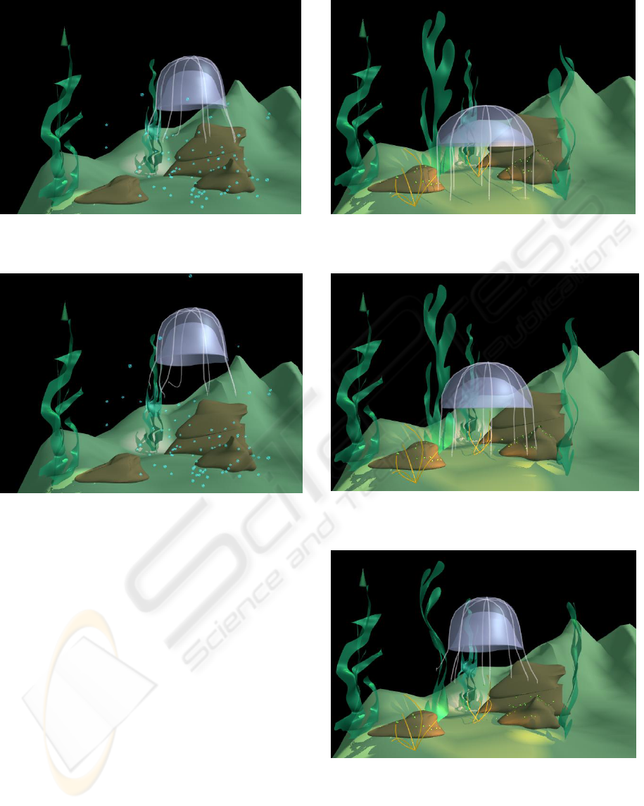
Figure 8 (c): Particles animated by jellyfish movement,
frame = 1400.
Figure 8 (d): Particles animated by jellyfish movement,
frame = 2000.
group of particles is intermixed by water flow.
Water movement also influences the tentacles. The
behavior of influenced objects looks quite natural.
In Fig.9, four screenshots from the underwater
scene with plants and some particles, placed in the
water, are shown; the video is joined to the article
and available on http://www.msi.unilim.fr/basilic
/Publications/2006/ATG06. The movement of the
green plants closest to the jellyfish can be easily
seen. In the underwater scene also appears the task
of a proper modeling of influenced objects. The
particle systems are well suited for this. Here, for
example, the green plants are modeled as particle
systems with particles placed in control points and
each particle is connected by springs with the closest
ones. Generally, this model should be complicated,
mostly by increasing the number of springs. In this
scene the simulation is visually pleasing and gives a
realistic impression of water flow pushing the plants.
Figure 9 (a): Underwater scene animated by jellyfish
movement, frame = 1.
Figure 9 (b): Underwater scene animated by jellyfish
movement, frame = 400.
Figure 9 (c): Underwater scene animated by jellyfish
movement, frame = 1400.
GRAPP 2006 - COMPUTER GRAPHICS THEORY AND APPLICATIONS
390

Figure 9 (d): Underwater scene animated by jellyfish
movement, frame = 2000.
5 CONCLUSIONS AND FUTURE
WORK
In this paper we presented a simplified physical
model, based on the Lattice-Boltzmann method, for
the simulation of a movement transformation from a
dynamic soft body to a liquid. It is applied to a
jellyfish in underwater scenes. The field is realized
as finite lattice surrounding a jellyfish.
The special boundary conditions on the body
surface are elaborated for this task. They are devoted
to the aim of visually realistic presentation of the
body motion transferring to the environment.
Attention is also paid to the simplicity of the model.
Compared to previous work in this domain, the
following points should be mentioned:
• The special boundary on the body surface,
which depends only on the local properties of
the surface. Independence of the boundary cells
from the rest lattice cells allows taking into
account the body as a generator of the motion.
• The modeling of body propagation in the
water.
In a future work, the implementation of body
trajectory changes, in order to avoid obstacles, can
be considered. This can be done as a function of an
obstacle bounding box coordinates and a body
bounding box coordinates. Some minimum distance
can be presented and, if needed, the correction
vector may be added to jellyfish transition at each
time step to keep this distance. Also, the full
interaction can be considered, the reciprocal
influence of the body and the liquid.
As a disadvantage, we can mention the possible
instability of the solution that is usual for liquid
modeling. The time step, the cell size, as well as the
coefficients for the LBM model should be properly
set in order to avoid instabilities.
REFERENCES
Guendelman, E., Selle, A., Losasso, F., Fedkiw, R.,
(2005). Coupling Water and Smoke to Thin
Deformable and Rigid shells. ACM Transactions on
Graphics 24(3)
, 973-981, (SIGGRAPH 2005).
Muller, M., Solenthaler, B., Keiser, R., Gross, M., (2005).
Particle-Based Fluid-Fluid Interaction.
Eurographics/ACM SIGGRAPH Symposium on
Computer Animation
, 1-7.
Foster, N., Metaxas, D., (1996). Realistic Animation of
Liquids. Graphical Models and Image Processing 58,
471-483.
Stam, J., 1999. Stable Fluids. ACM SIGGRAPH 99, 121-
128.
Foster, N., Fedkiw, R., (2001). Practical Animation of
Fluids.
Proceedings of SIGGRAPH, 23-30.
Genevaux, O., Habibi, A., Dischler, J., (2003). Simulating
Fluid-Solid Interaction. Graphics Interface, 31-38.
CIPS, Canadian Human-Computer Communication
Society, A K Peters, ISBN 1-56881-207-8, ISSN
0713-5424.
Carlson, M., Mucha, P., Turk, G., (2004). Rigid Fluid:
Animating the Interplay Between Rigid Bodies and
Fluid. ACM Trans. Graph. 23, 3, 377-384.
Muller, M., Charypar, D., Gross M., (2003). Particle-
Based Fluid Simulation for Interactive Application.
Proceedings of 2003 ACM SIGGRAPH Symposium on
Computer Animation
, 154-159.
Muller, M., Schrim, S., Teschner, M., Heidelberger, B.,
Gross, M., (2004). Interaction of Fluids with
Deformable Solids.
Journal of Computer Animation
and Virtual Worlds (CAVW) 15, 3-4
, 159-171.
Chen, S., Doolean, G., D., (1998). Lattice-Boltzmann
Method for Fluid Flows,
Ann. Rev. Fluid Mech., 30,
329-364.
Wei Li, Zhe Fan, Xiaoming Wei, Arie Kaufman, (2003,
Nov.). GPU-Based Flow Simulation with Complex
Boundaries Technical Report 031105, Computer
Science Department, SUNY at Stony Brook
.
(http://www.cs.sunysb.edu/~vislab/projects/amorphou
s/WeiWeb/hardwareLBM.htm)
Bhatnagar, P., L., Gross, E., P., Krook, M., (1954). A
model for collision processes in gases. I: small
amplitude processes in charged and neutral one-
component system. Phys. Rev. 94, 511–525.
Renwei Mei, Wei Shyy, Dazhi Yu, Li-Shi Luo, (2002).
Lattice Boltzmann Method for 3-D Flows with Curved
Boundary, NASA/CR-2002-211657 ICASE Report No.
2002-17.
McHenry, M., Jed, J., 2003. The ontogenetic scaling of
hydrodynamics and swimming performance in.
jellyfish (Aurelia aurita).
The Journal of Experimental
Biology
,(http://jeb.biologists.org/cgi/content/abstract/2
06/22/4125)
INTERACTION BETWEEN WATER AND DYNAMIC SOFT BODIES
391
