SPEEDING UP SNAKES
Enrico Kienel, Marek Van
ˇ
co and Guido Brunnett
Chemnitz University of Technology
Strae der Nationen 62, D-09107 Chemnitz, Germany
Keywords:
Active Contour Models, Snakes, Image Segmentation.
Abstract:
In this paper we summarize new and existing approaches for the semiautomatic image segmentation based
on active contour models. In order to replace the manual segmentation of images of the medical research of
the Center of Anatomy at the Georg August University of G
¨
ottingen we developed a user interface based on
snakes. Due to the huge images (sometimes bigger than 100 megapixels) the research deals with, an efficient
implementation is essential.
We use a multiresolution model to achieve a fast convergence in coarse scales. The subdivision of an active
contour into multiple segments and their treatment as open snakes allows us to exclude those parts of the
contour from the calculation, which have already aligned with the desired curve. In addition, the band structure
of the iteration matrices can be used to set up a linear algorithm for the computation of one single deformation
step. Finally, we gained an acceleration of the initial computation of the Edge Map and the Gradient Vector
Flow by the use of contemporary CPU architectures.
Furthermore, the storage of huge images next to additional data structures, such as the Gradient Vector Flow,
requires lots of memory. We show a possibility to save memory by a lossy scaling of the traditional potential
image forces.
1 INTRODUCTION
Imaging techniques have achieved a great importance
in many scientific domains, particularly in the med-
ical science. Whole series of digital photos are con-
sulted for the analysis of three-dimensional structures.
In order to reconstruct these three-dimensional mod-
els, it is necessary to perform an image segmentation.
In the framework of studying cellular events in the
embryonic development at the Georg August Univer-
sity of G
¨
ottingen, the segmentation of huge images
of serial histological sections is done manually in a
tedious process. We developed a user interface that
allows a semiautomatic segmentation of these images
based on active contours.
The snake model, first introduced by Kass (Kass
et al., 1987), offers a practical tool for the semiauto-
matic image segmentation. It combines many advan-
tages but features also some drawbacks which gave
reason for the publication of serveral improvements.
One major disadvantage is the necessity of initial-
izing a contour nearby the object’s edges due to the
narrow attraction range of the classical image en-
ergy. Kass proposed a convolution of the image with
a Gaussian kernel which slightly increases the cap-
ture range by blurring the original image. Rueck-
ert’s (Rueckert and Burger, 1996) multiscale approach
faces that problem by using different scales of the ker-
nel’s standard deviation. A balloon model was pro-
posed by Cohen (Cohen, 1991). Pressure forces along
the contour’s normals allow the inflation or the accel-
erated deflation of the snake. In order to increase the
attraction range of image edges Xu and Prince (Xu
and Prince, 1997) introduced an alternative image en-
ergy called Gradient Vector Flow. They calculate a
diffusion of the gradient vectors of a gray-level Edge
Map which additionally enables the active contour to
move into concave boundary regions. This is another
problem associated with the classical snake model.
The snake’s tendency of shrinking due to the for-
mulation of the internal energy terms discouraging the
stretching and bending behavior is sometimes stated
as a disadvantage, too. By applying Cohen’s balloon
model (Cohen, 1991) a snake is able to counteract the
contraction. Perrin (Perrin and Smith, 2001) proposed
alternative formulations of the internal energy which
323
Kienel E., Van
ˇ
co M. and Brunnett G. (2006).
SPEEDING UP SNAKES.
In Proceedings of the First International Conference on Computer Vision Theory and Applications, pages 323-330
DOI: 10.5220/0001362403230330
Copyright
c
SciTePress
also produce locally smooth curvatures and an evenly
spacing of the control points. In contrast to the tra-
ditional method this approach avoids shrinking and
pushing the model toward a straight line.
In (Mayer et al., 1997) ribbon snakes are proposed
for the road extraction in cartographic images, i.e. the
detection of thick lines with a significant width. A
ribbon snake is represented by a set of control points
on the centerline and a width at each point forming
two ribbon sides that are forced to be parallel. Ker-
schner (Kerschner, 2003) modifies this approach and
treats the two ribbon sides as separate snakes, called
twin snakes, with an additional attraction force among
each other which are thus relatively independent of
their initial position. This idea is similar to the dual
active contour model, published by Gunn (Gunn and
Nixon, 1997). In order to relax the sensitive choice of
parameters and the snake’s initialization nearby the
desired edges, they use two interlinked contours. One
contour expands from inside the target object while
the other one contracts from the outside. By the
means of an alternating deformation process the cou-
pled snakes try to reach the same equilibrium. That
way, even weak local minima can be rejected.
Ziplock snakes were introduced by Neuenschwan-
der (Neuenschwander et al., 1997). Only the two end
points of the open snake must be specified by the op-
erator, but exactly on the desired curve. The snake is
first approximated with a straight line between these
points. Beginning at the end points, gradually the
vertices are activated to optimize their position, i.e.
take part in the deformation process which is finished
when all vertices are movable and the snake stabilizes.
One further drawback of classical snakes is their
topological inflexibility. Geometric active contours,
developed independently by Caselles (Caselles et al.,
1993) and Malladi (Malladi et al., 1995), are based
on the theory of curve evolution and geometric flows.
Using a level set based implementation (Osher and
Sethian, 1988), the contours can easily split and
merge in the deformation process. A parametric ac-
tive contour model, that solves this problem, is the
topologically adaptable snake model, called T-Snake
which was presented by McInerney (McInerney and
Terzopoulos, 1995). There, a simplicial grid is super-
posed over the image domain which is used to iter-
atively reparameterize the deforming active contour,
also allowing a dynamical change in topology.
Due to the different problems associated with
snakes, an adaption of the model is required for each
special case. This paper summarizes some existing
approaches and some new aspects of speeding up the
snake deforming algorithm that are applied in our im-
plementation. It comprises a multiresolution strategy,
the use of multithreading techniques, subdividing the
snake into segments and a detailed description how to
compute one iteration step in O(n) instead of O(n
3
).
2 ACTIVE CONTOUR MODELS
A snake is a unit speed curve ~v : [0, 1]
R
→ R
2
with
~v(s) = (x(s), y(s))
T
that deforms on the spatial do-
main of an image by minimizing the following energy
functional:
E =
1
Z
0
1
2
α
∂~v
∂s
2
+ β
∂
2
~v
∂s
2
2
!
+E
ext
(~v)ds (1)
where α and β are positive weighting parameters. The
first two terms belong to the internal energy E
int
con-
trolling the smoothness of the snake while the external
energy E
ext
= E
img
+ E
con
consists of a potential
energy E
img
providing information about the image
and possibly a constraint energy E
con
.
The image energy E
img
defines a potential field
with low values at the desired image features. For
the edge extraction of an image I the following term
is often used (Xu and Prince, 1997):
E
img
(x, y) = −κ|∇(G
σ
(x, y) ∗ I(x, y))|
2
(2)
where G
σ
is a two-dimensional Gaussian function
with the standard deviation σ, ∇ is the gradient op-
erator and κ is a positive weighting parameter.
User interactions are often desirable to influence
the deformation, e.g. if an active contour is trapped
in a local energy minimum. Formulations of the con-
straint energy E
con
can be used to integrate an indi-
vidual behavior. Kass proposed user-defined points,
called springs and volcanos, that attract and push
away snakes. These points are useful instruments to
control a snake in the deforming process.
Using the calculus of variations a curve that mini-
mizes the integral (1) has to satisfy the Euler equation:
α
∂
2
~v
∂s
2
− β
∂
4
~v
∂s
4
− ∇E
ext
=
~
0 (3)
This is often taken as a force balance equation:
~
F
int
+
~
F
ext
=
~
0 (4)
with
~
F
int
= α
∂
2
~v
∂s
2
−β
∂
4
~v
∂s
4
and
~
F
ext
=
~
F
img
+
~
F
con
=
−∇E
ext
. Treating ~v as function of time and dis-
cretization of the equation (3) by approximating the
snake as a polygon and the partial derivatives as fi-
nite differences, a solution can be found iteratively as
follows (Kass et al., 1987):
~v
(t+1)
= (A+γI)
−1
(γ~v
(t)
−
~
F
img
(~v
(t)
)−
~
F
con
(~v
(t)
))
(5)
where ~v
(t)
is the vector of control points of the snake
at time step t, ~v
(t+1)
at time step t + 1 respectively,
A is a quadratic iteration matrix according to the di-
mension of the snake vector containing elements that
are linear combinations of α and β, I is the identity
matrix and γ is a positive weighting parameter con-
trolling the step size of each iteration which can be
considered as viscosity parameter.
VISAPP 2006 - IMAGE ANALYSIS
324
2.1 Extending Abilities
Due to the limited capture range of the image forces
and the sensitivity of local minima an initial contour
must be placed very close to the desired object bound-
aries. This is one of the most important disadvantages
of classical snakes.
One approach diminishing that problem was pub-
lished by Xu and Prince (Xu and Prince, 1997). The
replacement of the classical image force formulation
by a vector field, they called Gradient Vector Flow
(GVF), provides a larger attraction range by the pres-
ence of boundary information in homogeneous re-
gions. They define an Edge Map f(x, y) derived from
the image I(x, y) having large values at the features
of interest, e.g. image edges:
f(x, y) = |∇(G
σ
(x, y) ∗ I(x, y))|
2
(6)
Note, the field ∇f has vectors pointing to the image
edges, but still with a narrow capture range. The GVF
field ~g(x, y) = (u(x, y), v(x, y))
T
is calculated in the
next step by minimizing the energy functional:
E =
ZZ
µ(u
2
x
+u
2
y
+v
2
x
+v
2
y
)+|∇f |
2
|~g−∇f |
2
dxdy
(7)
The energy is dominated by the partial derivatives of
the vector field in homogeneous regions where |∇f |
is small, yielding a smooth field. |∇f| is large at im-
age edges and there E is minimal when ~g = ∇f . µ
is a positive weighting parameter which should be in-
creased the more noisy the image is. A possible way
to find a solution of equation (7) was described in (Xu
and Prince, 1998). Finally the potential force
~
F
img
in
equation (5) is replaced by the GVF term −~g.
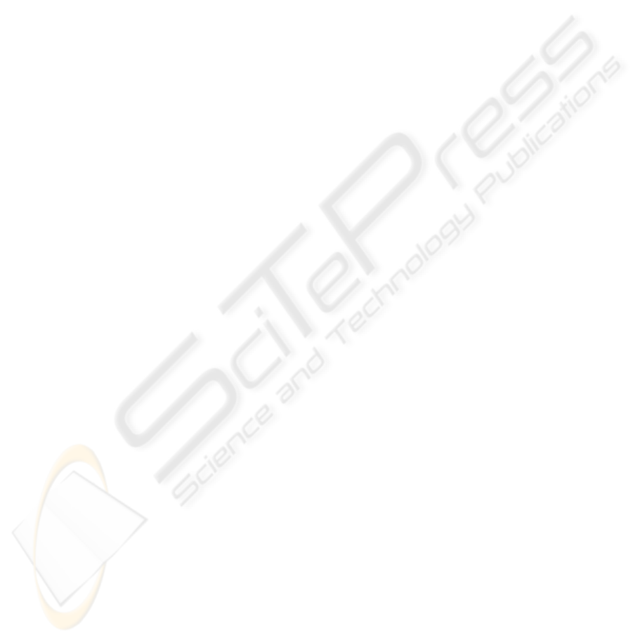
Figure 1 illustrates the diffusion of the image gradi-
ent considering a simple U-shaped object as example.
The enlarged attraction range of image edges sim-
plifies the active contour’s convergence into concave
boundary regions. Further on, the immediate close-
ness of initial contours to the desired object bound-
aries is not necessary any longer. But the advantages
of this method are bought dearly by the expensive
computation of the GVF field, especially with huge
images. We observed, GVF snakes produced more
qualitative results in our tests if a Gaussian filter was
applied to the image.
Cohen (Cohen, 1991) proposed a balloon model to
solve the problems encountered with the limited cap-
ture range of image edges while using the traditional
image energy. To allow an expansion of active con-
tours they introduced an inflation force:
~
F
p
= w
p
~n(s) (8)
where ~n(s) is the unit normal vector of the oriented
contour at the point ~v(s) and w
p
is a weighting pa-
rameter that controls the influence of that force. Ap-
plying this pressure force, as an additional part of the
(b)
(b)
(a) (b)
Figure 1: Image forces. (a) Traditional potential force field.
(b) Gradient Vector Flow field.
constraint forces
~
F
con
, the curve behaves like a bal-
loon, that is inflated. So it counteracts the snake’s
tendency to shrink under the predominant influence of
the elasticity force. Inflating active contours are also
able to detect closed object contours not only from
outside with the implicit aid of the shrinking behav-
ior but also from inside. Using this pressure force the
snake can easier move into concave boundary regions.
Changing the sign of w
p
makes the snake deflating
instead of inflating. An adequate choice of w
p
can
speed up the convergence process, particularly when
strong edges should be detected.
3 SPEEDING UP METHODS
This section describes the different methods for a fast
semiautomatic segmentation using snakes. The re-
search at the Georg August University of G
¨
ottingen
often deals with image sizes of more than 100
megapixels. Therefore an efficient implementation is
essential for a profitable practical use.
3.1 Acceleration of Initial
Computations
Once the potential image forces are determined, they
can be used for the entire segmentation process with-
out recalculation. In order to speed up the computa-
tion of the Edge Map and the GVF we take advantage
of current processor architectures that support the par-
allel execution of multiple arithmetical floating point
operations. However properly memory aligned data is
necessary for fast loading and storing instructions in
order to gain an noticeable acceleration. In fact load-
ing and storing time could slow down the computation
in spite of parallel execution due to unaligned data.
Further on, we use separate background threads for
their computation, particularly the GVF, which is very
SPEEDING UP SNAKES
325

time expensive for huge images like those from the re-
search in G
¨
ottingen. This saves a little time because
in the meantime the user is able to perform indepen-
dent tasks like setting up one or more initial contours
or adjusting parameter values.
3.2 Multiresolution with an
Automation Approach
We use a multiresolution approach which is very sim-
ilar to Leroy (Leroy et al., 1996). After a huge im-
age has been loaded several smaller scales of the im-
age are computed. Each scale has half the width
and height of the above scale. This computation is
repeated until the coarsest image size is about one
megapixel.
Starting with a rough initial contour with a few
points in the coarsest scale, we can set up an iter-
ative process. By solving small systems of linear
equations our approach determines a suitable solu-
tion curve very rapidly. Furthermore, the tendency to
shrink is stronger if the active contour has only a few
points, due to the structure of the internal forces, i.e.
the snake needs less iterations. A simple polygonal
initialized snake is filled with many collinear points
on the edges of the polygon. If these points are lo-
cated in regions without a potential image force they
have a minimal energy. So they will not move unless
a discrete curvature is present which can be found,
of course, at the polygon’s vertices. That means that
these vertices are the first deforming parts of the snake
spreading a smaller curvature to their neighbors. One
can imagine that the snake is shrinking faster the less
points it has. In fact, this behavior can be desired,
though it is commonly seen as a disadvantage. Often,
a snake has to move across regions without any edge
information when detecting object boundaries from
outside by contraction. Therefore, it has to deform
while being exposed only to the internal forces.
In order to keep an approximate point distance, new
points are inserted when switching to a higher resolu-
tion next to scaling the contour to an appropriate size.
That means the result of the last lower scale is used
as the initial curve for the current scale. When the
original resolution is reached the snake should be al-
ready very close to the desired curve and therefore
only a few iterations are needed for a more detailed
extraction. This approach leads to an acceleration,
because the biggest distance of the contour is covered
in coarse scales with only a few points and in higher
scales just minimal refinements are needed.
User interaction can be further reduced if accept-
able results can be achieved without the need of pa-
rameter adjustments during the deforming process.
Based on that multiresolution strategy, we have de-
signed an automation technique, that allows an auto-
matic image segmentation for images with a sufficient
quality. We start with a given initial contour in the
coarsest scale with the traditional image forces (no
GVF). Besides we use the opposite image forces for
the beginning convergence process, i.e. using
~
F
img
instead of −
~
F
img
in equation (5). That way, we can
keep the snake slightly distant from the desired object
boundaries. Otherwise we observed the contour of-
ten moving across weak edges in lower scales. The
deformation procedure automatically switches to the
next scale after the snake has stabilized its position.
It is scaled to double size and additional points are
inserted. For each reached scale the potential im-
age forces are recomputed, according to the new size.
These steps are repeated until we reached the original
size of the image. Then the classical image energy
(with the correct sign) or the GVF field is used for
the last time the deforming process gets started. Con-
verged close to the desired edges in the meantime the
snake can now fit to them very quickly.
3.3 Using Segments
Kerschner (Kerschner, 2003) proposed an approach
that uses segments in order to overcome local min-
ima. A traffic light system enables the snake to diag-
nose the quality of the segmentation result of itself.
Thereby segments in different colors (red for rejected
results, yellow for unsure results, green for trustwor-
thy results) are presented to the operator who can in-
fluence the accepting procedure of the automatic rat-
ing system. Typically, yellow and red parts are linked
and deform afterward with a modified energy func-
tion, e.g. by changing parameter values.
We use segments to gain another acceleration. Dur-
ing the deforming process parts of a snake often reach
the desired object boundaries faster than others, e.g.
an active contour has not moved into an concave
boundary region yet while the rest of the object has
been detected already. Points in these parts will not
move anymore and thus can be excluded from the it-
erative minimization procedure. This can be done by
subdividing the snake into segments and treating them
as open snakes.
The segmentation process is started with one seg-
ment – one closed contour. The movement of each
point of the snake is traced for the last few iterations.
If the position of several adjacent points does not
change significantly within that time, two segments
are formed. The first segment contains these adja-
cent points and is locked, i.e. is ignored in the future
minimization process. The second segment is filled
with the remaining points and further on deforming
as open snake by solving a respectively smaller sys-
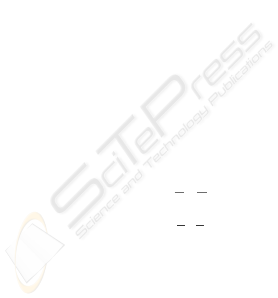
tem of equations. Figure 2 shows the use of segments.
VISAPP 2006 - IMAGE ANALYSIS
326
(a) (b) (c)
Figure 2: Segments. (a) Rough initial contour. (b) First
segments are formed. (c) Approximately 90% of the desired
curve are already detected. Only 10% of the vertices are
included in the computation.
3.4 Fast Implementation
For the computation of one single iteration step a
system of linear equations (Kass et al., 1987) has to
be solved. We write the system (5) as ~y = B~x.
B ∈ R
n×n
is a sparse matrix with a band structure
for both closed and open snakes where n is the num-
ber of control points of the snake. In this section we
describe an efficient O(n) algorithm to solve that sys-
tem for both cases.
We assume α and β being constant along the whole
curve. According to the definition of finite differ-
ences, we set:
a := β
b := −α − 4β
c := 2α + 6β + γ
3.4.1 Closed Snakes
In compliance with cyclic boundary conditions, i.e.
the knot vector ~v of the contour is periodically con-
tinued, all finite differences are computable. Thus, B
has the shape:
B =
c b a a b
b c b
.
.
.
a
a b c
.
.
.
a
.
.
.
.
.
.
.
.
.
b a
a b c b a
a b
.
.
.
.
.
.
.
.
.
a
.
.
.
c b a
a
.
.
.
b c b
b a a b c
We now subdivide the symmetric matrix B as follows:
B =
E F
F
T
H
(9)
where E ∈ R
(n−2)×(n−2)
, F ∈ R
(n−2)×2
and H ∈
R
2×2
are also matrices and E is invertible. Note E
is really pentadiagonal. With the Schur complement
S := H − F
T
E
−1
F of E in B we can factorize the
matrix:
B =
E 0
F
T
S
I E
−1
F
0 I
(10)
where I is the identity matrix of an appropriate size.
In order to solve the system ~y = B~x in O(n), we
perform the following steps.
1. Compute Cholesky’s decomposition of the matrix
E = LL
T
in O(n) (see algorithm 1 in the appen-
dix). Note, L is a lower triangular matrix and has
the lower bandwidth 2, i.e. l
ij
= 0 as i > j + 2.
2. Compute the matrix Q
0
of the equation LQ
0
= F .
A solution of that matrix equation can be found by
solving the systems L~q
0
i
=
~
f
i
, (i = 1, 2) by an
optimized forward substitution in O(n) (see algo-
rithm 2 in the appendix) where ~q
0
i
and
~
f
i
are the
i-th column vectors of Q
0
and F .
3. Compute the matrix Q of the equation L
T
Q = Q
0
the same way by an optimized backward substitu-
tion in O(n) (analogous to forward substitution).
Now Q = E
−1
F is determined.
4. Compute the Schur complement S = H − F
T
Q.
Now we split the vector ~x = [~x
1
, ~x
2
]
T
, where ~x
1
∈
R
(n−2)
and ~x
2
∈ R
2
. All other vectors are split anal-
ogous, yielding with equation (10):
E 0
F
T
S
I Q
0 I
~x
1
~x
2
=
~y
1
~y
2
For the determination of ~x, some steps remain:
5. Compute ~w
1
by solving E ~w
1
= ~y
1
.
6. Set ~w
2
= ~y
2
− F
T
~w
1
.
7. Compute ~x
2
by solving S~x
2
= ~w
2
.
8. Set ~x
1
= ~w
1
− Q~x
2
.
Finally, the solution of B~x = ~y is determined. Note,
the steps 1–4 are only needed if one of the parameters
or the size of the system (n) changes by the inser-
tion or deletion of vertices. The steps 5–8 have to be
performed after each iteration. The complexity of all
steps is O(n), except the steps 6 and 7 which can be
computed in O(1). Thus, the overall complexity for
all steps is O(n).
3.4.2 Open Snakes
Open snakes need other boundary conditions. We re-
peat twice the first vertex at the beginning and the last
vertex at the end of the snake’s knot vector ~v. Again,
all finite differences are computable. Now the matrix
SPEEDING UP SNAKES
327

B has the following shape:
B =
˜c b a
˜
b c b
.
.
.
a b c
.
.
.
a
.
.
.
.
.
.
.
.
.
b a
a b c b a
a b
.
.
.
.
.
.
.
.
.
a
.
.
.
c b a
.
.
.
b c
˜
b
a b ˜c
where ˜c = a + b + c and
˜
b = a + b. Note, B
is not symmetric anymore and thus, we cannot use
Cholesky’s decomposition. Instead, we can use an
optimized LU decomposition of B = LU , because
B is completely pentadiagonal. Then, the solution of
the system B~x = ~y can be found as follows:
1. Compute the LU decomposition of B = LU in
O(n) (see algorithm 3 in the appendix). Note, L
is again a lower triangular matrix with the lower
bandwidth 2, and U is an upper triangular matrix
respectively with the upper bandwidth 2.
2. Compute ~w by solving L~w = ~y using again an op-
timized forward substitution.
3. Compute ~x by solving U ~x = ~w using again an op-
timized backward substitution.
The LU decomposition has to be recomputed each
time the parameters or the number of vertices change.
All of the steps have a linear complexity and thus, the
overall computation has the complexity O(n), too.
3.5 Memory Saving by Scaling
The semiautomatic segmentation of huge images us-
ing snakes needs a lot of memory, especially for the
precalculation of the image’s potential energy, such as
the traditional image energy or the GVF. However, it
is desirable, that the image next to all necessary data
structures fits into physical memory.
We store the Edge Map and the Edge Map’s gra-
dient internally scaled in a lossy format in order to
be able to handle larger images. In either case, the
Edge Map gradient will be needed, because it is the
starting point for the GVF computation and also the
traditional image forces can be derived directly from
it. Typically, floating point values use 32 bit for single
or 64 bit for double precision. We only use 16 bit.
Let x
i
∈ [x
min
, x
max
], i = 1, . . . , n be n floating
point values. In order to represent these values using
16 bit, they can be scaled to integer values of the in-
terval [0, 65535] using the encoding function f
e
and
the decoding function f
d
:
f
e
(x
i
) =
x
i
− x
min
x
max
− x
min
· 65535
(11)
f
d
(y
i
) =
y
i
65535
· (x
max
− x
min
) + x
min
(12)
x
min
and x
max
must be stored as 32 bit or 64 bit float-
ing point values, while the storage of the n integer
values y
i
only needs 16 bit each with.
The storage of the Edge Map needs one and its gra-
dient two floating point values per pixel. Using the
introduced scaling method we save 3 bytes per pixel.
Considering an image with 100 megapixels, we would
save 300 MB.
Of course, that approach slows down the computa-
tion of these structures, because at the beginning the
minimal and maximal values have to be determined
and elements need to be decoded in order to access
them. That is why this method was not applied to
the GVF, because the permanent encoding, decoding
and redetermination of x
min
and x
max
slowed down
its computation disproportionately, while the deceler-
ation, caused by the implementation for the Edge Map
and its gradient, is tolerable.
This technique leads to another speedup, because a
larger amount of data can be kept in physical memory,
instead of swapping out portions on a slow secondary
storage when reaching the memory limit.
4 RESULTS
Synthetic situations were created, to test the different
speeding up methods.
1
We optimized our implementation by the use of
SSE
TM
instructions. Due to the memory alignment
condition, these techiques were not applied to all cal-
culations. Actually, the time for the determination of
the Edge Map and the GVF could be considerably de-
creased to approximately 30%.
Table 1 points out the importance of an optimized
implementation. It shows the time of a naive O(n
3
)
implementation of the solution of the system (5) us-
ing the LU decomposition, confronting the optimized
O(n) version, described in section 3.4.
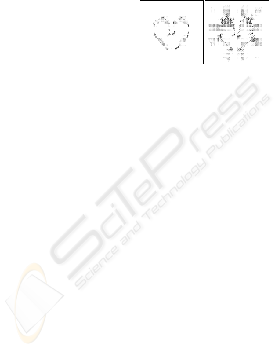
Figure 3 shows a histological section of the re-
search in G
¨
ottingen with the original size of 3900 ×
4120 pixels. The time for achieving the result (3b),
was measured in different scales of the same image,
starting from the same initial contour (3a), but with
different number of vertices respectively. The results
are presented in table 2.
1
All results were achieved on an Intel Pentium IV
2.4GHz processor with 1GB DDR-RAM.
VISAPP 2006 - IMAGE ANALYSIS
328

Table 1: Comparison between naive and optimized imple-
mentation. 1000 deforming steps were calculated in each
case. The times neither include the costs of the precompu-
tation of the Edge Map nor the costs for the GVF.
vertices O(n
3
) O(n) factor
256 1 min 36 s 4.8 s 20
512 23 min 25 s 8.6 s 166
1024 6 h 28 min 11.2 s 2079
2048 - 22.4 s -
4096 - 52.8 s -
(a) (b)
Figure 3: A histological section scaled at
1
8
size. (a) Rough
initial contour. (b) Deformation to the approximate convex
hull of the object.
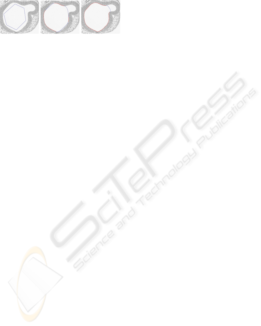
Finally, the introduced techniques were applied to
detect the outer contour of the object of the histo-
logical section in figure 4a. The image with a size
of 9100 × 15965 pixels was preprocessed with some
image filters and scaled to 3376 × 5923 pixels (4b)
so that the GVF and the image itself fit into mem-
ory. The final contour (4c), has 1555 vertices and was
achieved after 2 minutes and 15 seconds and 5660 it-
erations (without the computational time for the po-
tential forces). Assuming two vertices per second
can be set by hand, a manual segmentation would
have taken approximately 15 minutes. The deform-
ing process comprises four image scalings and a fine
tuning of the result by the insertion of some springs.
5 CONCLUSION
In this article, we presented different methods of
speeding up the semiautomatic image segmentation
process using parametric active contour models. Aim-
ing the replacement of the tedious manual segmen-
tation by a faster semiautomatic segmentation for
the medical research at the University of G
¨
ottingen,
we developed a graphical user interface combining
these techniques with other improving approaches
Table 2: Times and deforming steps to achieve the result of
figure 3b in different scales.
scale vertices iterations time
12.5% 130 563 1.1 s
25% 240 2113 10.5 s
50% 480 8867 1 min 20 s
100% 950 35269 10 min 5 s
(a) (b) (c)
Figure 4: (a) Original image. (b) Filtered and scaled image
with initial contour. (c) Final result after interactions.
that were already published, such as the Gradient Vec-
tor Flow and the balloon model which are popular
extensions of the traditional snake model providing a
larger attraction range. This research deals with huge
images and thus an efficient and memory saving im-
plementation is desirable to justify the practical appli-
cation.
It was shown how important it is, to take advantage
of the band structure of the underlying matrices. Also
the multiresolution method leaded to a considerable
acceleration due to the fast convergence in coarser
scales. Using segments is advantageous for the fi-
nal refinement steps, e.g. in the original scale of the
image where many successfully detected parts of the
snake can be excluded from the calculation.
Because of dealing with those huge images, mem-
ory saving approaches are also very important, like
the scaling of the values of the traditional potential
energy. Further approaches reducing the memory us-
age would be useful, especially for the storage of the
Gradient Vector Flow.
APPENDIX: ALGORITHMS
All of the shown algorithms were used to achieve
O(n) complexity for one single iteration step.
SPEEDING UP SNAKES
329

Algorithm 1: Efficient Cholesky decomposition
Input : Symmetric band matrix A = (a
ij
)
n,n
i=1,j=1
with the bandwidth w.
Output : Cholesky decomposition of the matrix
A = LL
T
. A will be overwritten with the
elements of the matrix L.
w
l
←
w
2
for i ← 1 to n do
a
ii
← a
ii
−
i−1
k=max{1,i−w
l
}
a
ik
for j ← i+1 to min{i+w
l
, n} do
a
ji
←
1
a
ii
a
ij
−
i−1
k=max{1,j−w
l
}
a
ik
a
jk
end
end
Algorithm 2: Efficient forward substitution
Input : Lower triangular matrix L = (l
ij
)
n,n
i=1,j=1
with the lower bandwidth w
l
, result vector
~
b = (b
1
, . . . , b
n
)
T
.
Output : Solution vector ~x = (x
1
, . . . , x
n
)
T
of the
system L~x =
~
b.
for i ← 1 to n do
x
i
←
1
l
ii
b
i
−
i−1
j=max{1,i−w
l
}
l
ij
x
j
end
Algorithm 3: Efficient LU decomposition
Input : Band matrix A = (a
ij
)
n,n
i=1,j=1
with the
lower and upper bandwidth w
l
and w
u
.
Output : LU decomposition of the matrix A = LU.
A will be overwritten with elements of the
lower triangular matrix L below and with
elements of the upper triangular matrix U
above of and upon the main diagonal.
for k ← 1 to n do
for i ← k+1 to min{k+w
l
, n} do a
ik
←
a
ik
a
kk
for j ← k+1 to min{k+w
u
, n} do
for i ← k+1 to min{k+w
l
, n} do
a
ij
← a
ij
− a
ik
a
kj
end
end
end
REFERENCES
Caselles, V., Catte, F., Coll, T., and Dibos, F. (1993). A geo-
metric model for active contours. Numerische Mathe-
matik, 66:1–31.
Cohen, L. D. (1991). On active contour models and bal-
loons. CVGIP: Image Understanding, 53(2):211–218.
Gunn, S. R. and Nixon, M. S. (1997). A robust snake im-
plementation; a dual active contour. IEEE Transac-
tions on Pattern Analysis and Machine Intelligence,
19(1):63–68.
Kass, M., Witkin, A., and Terzopoulos, D. (1987). Snakes:
Active contour models. International Journal of Com-
puter Vision, 1(4):321–331.
Kerschner, M. (2003). Snakes f
¨
ur Aufgaben der digi-
talen Photogrammetrie und Topographie. Disserta-
tion, Technische Universit
¨
at Wien.
Leroy, B., Herlin, I. L., and Cohen, L. D. (1996). Multi-
resolution algorithms for active contour models. In
Proceedings of the 12th International Conference
on Analysis and Optimization of Systems Images,
Wavelets and PDE’S, Rocquencourt (France).
Malladi, R., Sethian, J. A., and Vemuri, B. C. (1995).
Shape modeling with front propagation: A level set
approach. IEEE Transactions on Pattern Analysis and
Machine Intelligence, 17(2):158–175.
Mayer, H., Laptev, I., Baumgartner, A., and Steger, C.
(1997). Automatic road extraction based on multi-
scale modeling, context, and snakes. In Theoretical
and Practical Aspects of Surface Reconstruction and
3-D Object Extraction, volume 32, Part 3-2W3, pages
106–113.
McInerney, T. and Terzopoulos, D. (1995). Topologically
adaptable snakes. In Fifth International Conference
on Computer Vision, pages 840–845. IEEE Computer
Society.
Neuenschwander, W. M., Fua, P., Iverson, L., Szkely, G.,
and K
¨
ubler, O. (1997). Ziplock snakes. International
Journal of Computer Vision, 25(3):191–201.
Osher, S. and Sethian, J. A. (1988). Fronts propagating
with curvature-dependent speed: algorithms based on
hamilton-jacobi formulations. Journal of Computa-
tional Physics, 79(1):12–49.
Perrin, D. P. and Smith, C. E. (2001). Rethinking classical
internal forces for active contour models. In IEEE In-
ternational Conference on Computer Vision and Pat-
tern Recognition, pages II: 354–359.
Rueckert, D. and Burger, P. (1996). A multiscale approach
to contour fitting for mr images. In SPIE Confer-
ence on Medical Imaging: Image Processing, volume
2710, pages 289–300. SPIE.
Xu, C. and Prince, J. L. (1997). Gradient vector flow: A new
external force for snakes. In Proceedings of the 1997
Conference on Computer Vision and Pattern Recogni-
tion (CVPR ’97), pages 66–71. IEEE Computer Soci-
ety.
Xu, C. and Prince, J. L. (1998). Snakes, shapes, and gra-
dient vector flow. In IEEE Transactions on Image
Processing, pages 359–369. IEEE Computer Society.
VISAPP 2006 - IMAGE ANALYSIS
330
