MOTION SEGMENTATION THROUGH FACTORIZATION -
APPLICATION TO NIGHT DRIVING ASSISTANCE
Carme Juli
`
a, Joan Serrat, Antonio L
´
opez, Felipe Lumbreras and Dani Ponsa
Computer Vision Center and Computer Science Department
Universitat Aut
`
onoma de Barcelona
08193 Bellaterra, Spain
Thorsten Graf
Volkswagen AG Group Research, Electronics
Wolfsburg, D-38436
Keywords:
driving assistance, motion segmentation, factorization.
Abstract:
Intelligent vehicles are those equipped with sensors and information control systems that can assist human
driving. In this context, we address the problem of detecting vehicles at night. The aim is to distinguish vehi-
cles from lamp posts and traffic sign reflections by grouping the blob trajectories according to their apparent
motion. We have adapted two factorization techniques, originally designed to estimate the scene structure
from motion: the Costeira–Kanade and the Han–Kanade, named after their authors. Results on both vehicle
existence in the field of view and motion segmentation are reported.
1 INTRODUCTION
We focus our work in detecting vehicles at night from
video sequences when they are far away or at a mid-
range distance. One possible application would be to
define an intelligent lighting system, that includes au-
tomatic high and low beam switching. The aim is to
distinguish vehicles from lamp posts and traffic sign
reflections. To this end, we try to check whether there
are two or more motions in a sequence, or just one.
In the first case, at least one of the motions must be
a vehicle, since the rest correspond to static features
and/or other vehicles. In the second case, we can not
decide just on the ground of motion, but other cues
should be used, like size change over time or location
in the image.
Our approach is to group trajectories of fea-
ture points according to their apparent motion. In
(Megret and DeMenthon, 2002), a taxonomy of
spatio-temporal techniques is presented. One of these
techniques is factorization. This is a theoretically
sound method addressing the structure from motion
problem: recovering both 3D scene shape and camera
motion from trajectories of tracked features. Since
the camera motion can be made relative to each of the
scene objects, it can be employed for motion segmen-
tation, by grouping those features whose 3D motion
is similar.
Factorization has some distinct advantages over
other structure from motion approaches: it requires
just one camera, not necessary calibrated, and there
is no need to know the number of objects to recon-
struct, nor to a priori group the features according to
the object they belong to.
However, this technique has some restrictions: a
certain number m of features have to be tracked along
the same n frames, giving rise to m complete and si-
multaneous trajectories of length n. There is a mini-
mum number of features and frames required, which
depend on the specific factorization technique, and
the camera is usually approximated either by an or-
thographic or an affine projection.
The central idea of all factorization techniques is
the ability to express a matrix W containing the fea-
ture trajectories as the product of two unknown matri-
ces W = MS, namely, the objects 3D shape S and the
relative camera pose at each frame M. Although un-
known, they can be estimated thanks to the key result
that their rank is small and to constraints derived from
the orthonormality of the camera axes. The exact rank
of M and S and the specific constraints depend on the
particular factorization technique at hand, as we will
see in short.
The camera model used is the basis of all factoriza-
tion methods. Kanatani and Sugaya rightly pointed
out in a review paper (Kanatani and Sugaya, 2004)
270
Julià C., Serrat J., López A., Lumbreras F., Ponsa D. and Graf T. (2006).
MOTION SEGMENTATION THROUGH FACTORIZATION - APPLICATION TO NIGHT DRIVING ASSISTANCE.
In Proceedings of the First International Conference on Computer Vision Theory and Applications, pages 270-277
DOI: 10.5220/0001362802700277
Copyright
c
 SciTePress

that there is still a wide–spread misunderstanding that
factorization is a method for 3D reconstruction us-
ing SVD, whereas the underlying principle is only
the affine approximation to camera imaging. SVD
is just a mean for numerically computing the least–
squares solution. Actually, factorization is a family of
methods, the original one based on the simplest affine
camera model —orthographic projection—, and sub-
sequent methods on increasingly more accurate mod-
els: scaled orthographic projection, weak perspective,
para–perspective and the full perspective camera.
Other techniques applied to vehicle detection from
a moving observer have been recently published
(Woelk, 2004; Hu, 1999). Both are based on the es-
timation of the focus of expansion (FOE) due to the
translation component of the camera motion. They
can not be applied to our night sequences, because
very few or no static feature pairs are present in order
to calculate the FOE. Besides, due to the pitch and
yaw motion of the car, the trajectories of the points
are not straight and that makes the FOE estimation
difficult.
This paper is organized as follows. In sections 2
and 3 we introduce two factorization formulations. In
section 4 we show how to adapt them to the vehicle
detection problem. Section 5 contains the results, and
we end with the conclusions and future work in sec-
tion 6.
2 THE MULTI–BODY CASE
The seminal factorization work for structure from mo-
tion by Tomasi and Kanade (Tomasi and Kanade,
1992) was formulated for a single static rigid object
viewed by a moving camera. Instead, the Costeira
and Kanade formulation (Costeira and Kanade, 1998)
of the factorization method assumes one or more
moving objects viewed by a static camera. Accord-
ing to the later, let be p
j
, j = 1...m the 3D object
points expressed in some arbitrary coordinate sys-
tem fixed to the object. In homogeneous coordinates,
s
j
=

p
j
1

t
. At each time i = 1...n, these points
are projected into the image according to the simple
orthographic camera model:
u
ij
= i
t
i
p
j
+t
xi
v
ij
= j
t
i
p
j
+t
yi
(1)
being i
i
,j
i
the camera axes and (t
xi
,t
yi
) its translation.
All image trajectories (u
ij
,v
ij
) are stacked into a
2n × m measurement matrix W, which, according to
equation (1), is factored as the product of the shape
and motion matrices we want to calculate:
⎡
⎢
⎢
⎢
⎢
⎢
⎢
⎢
⎣
u
11
... u
1m
.
.
.
.
.
.
u
n1
... u
nm
v
11
... v
1m
.
.
.
.
.
.
v
n1
... v
nm
⎤
⎥
⎥
⎥
⎥
⎥
⎥
⎥
⎦
=
⎡
⎢
⎢
⎢
⎢
⎢
⎢
⎢
⎣
i
t
1
t
x1
.
.
.
.
.
.
i
t
n
t
xn
j
t
1
t
y1
.
.
.
.
.
.
j
t
n
t
yn
⎤
⎥
⎥
⎥
⎥
⎥
⎥
⎥
⎦
[s
1
s
2
... s
m
]
W = MS (2)
In the absence of noise, the rank of W is at most 4.
The SVD decomposition W = U
2n×4
Σ
4×4
V
t
4×m
yields
the true M and S but for an unknown invertible matrix
A
4×4
: W = MS =
ˆ
MAA
−1
ˆ
S, with
ˆ
M = UΣ
1
2
,
ˆ
S = Σ
1
2
S.
Fortunately, A can be computed through a so called
normalization process by using the fact that the rows
of M represent the camera rotation axes and satisfy,
for i = 1...n, the following conditions:
i
t
i
· i
i
= j
t
i
· j
i
= 1
i
t
i
· j
i
= 0 (3)
If the scene contains p objects moving indepen-
dently, each with a certain number of features, the
matrix of all trajectories sorted by object W
∗
factor-
izes as before into the product of p block matrices M
k
and S
k
, k = 1... p. But, of course, we do not know
W
∗
, because features are not sorted by object, which
is precisely what we want to obtain from the motion
segmentation. Instead, W is equal to W
∗
but having
permuted some columns.
The main finding of the Costeira–Kanade’s method
is the so called shape interaction matrix:
Q
∗
= V
∗
V
∗t
(4)
This matrix has an interesting block–diagonal
structure and, if features k and l belong to different
objects, Q
∗
kl
is zero. The key point is that this is also
true even though the trajectories are not sorted by ob-
ject: since W is equal to W
∗
but having permuted
some columns, so V
t
is equal to V
∗t
only that permut-
ing the same set of columns. Therefore, Q
∗
will result
by permuting rows and columns of Q in the same way.
The shape from motion problem for multiple mov-
ing objects has been reduced to that of finding out
the right row and column permutations of Q such that
it becomes block–diagonal, because then, the single
body algorithm can be applied. However, recover-
ing Q
∗
from Q, and thus performing feature grouping
(motion segmentation), is still a tough problem be-
cause noise makes the entries of Q corresponding to
features of different objects not exactly zero.
Costeira and Kanade present a two–steps method to
determine the diagonal blocks of Q
∗
from Q. Firstly,
Q needs to be sorted so that its structure resembles
as much as possible a block diagonal matrix. They
MOTION SEGMENTATION THROUGH FACTORIZATION - Application to Night Driving Assistance
271

propose a simple greedy algorithm for this search.
Secondly, the bounds of each block have to be deter-
mined. This is a necessary step to decide how many
independent motions are there and which features be-
long to each one. An energy function is defined both
to find potential block limits and to choose the motion
segmentation solution:
ε (l)=
l
∑
i=1
l
∑
j=1
(Q
∗
ij
)
2
, l = 1...m (5)
3 LINEARLY MOVING
MULTIPLE OBJECTS
The algorithm of Han and Kanade (Han and Kanade,
2004) deals with a moving camera and multiple static
or dynamic objects, but now constrained to move in
linear trajectories and at constant speeds. Recall that
this is a reasonable assumption for small intervals of
time.
In a certain world coordinate system, any point p
ij
,
j = 1...m is represented by
p
ij
= s
j
+ iv
j
(6)
where s
j
is the position of the j-th feature at frame 0,
v
j
is its motion velocity and i = 1...n is the frame
number. Again, the image trajectories obtained with
the orthographic camera model are stacked in the ma-
trix W:
W =
⎡
⎢
⎢
⎢
⎢
⎣
u
11
u
12
... u
1m
v
11
v
12
... v
1m
.
.
.
.
.
.
.
.
.
u
n1
u
n2
... u
nm
v
n1
v
n2
... v
nm
⎤
⎥
⎥
⎥
⎥
⎦
(7)
As before, this matrix is factored as the product of
the shape and motion matrices. Now, the rank is 6
since we assume m,n ≥ 6 and S has 6 rows:
W
2n×m
= M
2n×6
S
6×m
+ T
2n×1
[
11... 1
] (8)
where
M =
⎡
⎢
⎢
⎢
⎢
⎣
i
t
1
1i
t
1
j
t
1
1j
t
1
.
.
.
.
.
.
i
t
n
ni
t
n
j
t
n
nj
t
n
⎤
⎥
⎥
⎥
⎥
⎦
(9)
S =

s
1
s
2
... s
m
v
1
v
2
... v
m

(10)
T =[
t
x1
t
y1
... t
xn
t
yn
]
t
(11)
By moving the world coordinate system to the cen-
troid of all the p
ij
at each frame, it is possible to ob-
tain T and subtract it from the matrix W, obtaining
ˆ
W
2n×m
=
ˆ
M
2n×6
ˆ
S
6×m
. The coordinate system moves
as its origin p
ij
linearly with constant speed v
c
and the
static points have the same velocity, but with changed
sign. Therefore, in order to obtain v
j
in a fixed coor-
dinate system, we must subtract v
c
to v
j
.
In the absence of noise, the rank of
ˆ
W is at
most six and M and S are obtained from its SVD:
ˆ
W = U
2n×6
Σ
6×6
V
t
6×m
. Again, this decomposition is
up to an affine transformation A
6×6
:
ˆ
W =
ˆ
MAA
−1
ˆ
S =
MS, which can be computed with a normalization
process similar to that of section 2.
4 VEHICLE DETECTION
THROUGH FACTORIZATION
4.1 Trajectory Grouping Through
Multibody Factorization
Two scenarios are possible with regard the content of
a sequence:
1. Only one type of motion is present, that is, all
features belong to a unique group or object. In this
case we can not yet decide whether they are static or
dynamic.
2. At least two types of motion can be differenti-
ated. Then, it is clear that at least one of them is a
moving vehicle.
Accordingly, two strategies are possible following
the Costeira–Kanade method:
1. Inspect the obtained Q
∗
and the list of possi-
ble block limits just to decide whether there is just
one group formed by all the features or instead two or
more groups are more likely.
2. Perform motion segmentation in order to group
all features into independently moving objects.
The first one answers if there are two or more ve-
hicles, whereas the second one tells which of the fea-
tures correspond to vehicles and which ones to static
lights. Of course, the later is a much more interesting
question but also more difficult to answer reliably.
In both cases, it is necessary to know a priori, or
else estimate, the true rank r of W in order to com-
pute Q
∗
= V
∗
V
∗t
. We are thus going to select the r
for which the resulting Q
∗
achieves the most block-
like structure. Hopefully, if there is just one mov-
ing object, any value of r will not achieve a sufficient
block–diagonal matrix, according to a certain blocki-
ness measure we have to design. Otherwise, we want
this measure to attain its maximum for the right r.
However, we must first bound the range of values for
the rank of W.
VISAPP 2006 - MOTION, TRACKING AND STEREO VISION
272

One key assumption of the Costeira–Kanade
method is not often satisfied in practice in traffic se-
quences: that objects move independently. The mo-
tion matrix M
k
for each object k is of the form:
M
k
=
⎡
⎢
⎢
⎢
⎢
⎢
⎢
⎢
⎢
⎣
i
t
1,k
t
x1
.
.
.
.
.
.
i
t
n,k
t
xn
j
t
1,k
t
y1
.
.
.
.
.
.
j
t
n,k
t
yn
⎤
⎥
⎥
⎥
⎥
⎥
⎥
⎥
⎥
⎦
(12)
Our road sequences are around just one or two sec-
onds. During these short time intervals, vehicles do
not rotate by themselves but for lane changes and road
curves. However, it can hardly be appreciated due to
the usually large distance to the camera. Nevertheless,
there is always a continuous and oscillating relative
rotation with respect the camera, caused by the pitch
motion of the car to which it is attached. Since this ro-
tation is the same for all objects, I
k
=[i
1,k
... i
n,k
] and
J
k
=[j
1,k
... j
n,k
] are equal for each k = 1...p. Thus,
the rank of M is reduced to 3 plus the number of lin-
early independent translation vectors t
k
. At this point,
we introduce the following simplifying assumptions:
every vehicle appears, at least, as two blobs (fea-
tures), and in any sequence at least m = 4 features
are tracked. Consequently, the maximum number of
objects is p = 
m
2
 and, in theory, the rank of W lies
within the range
4 ≤ r ≤ min(m,3+

m
2

) (13)
Translation vectors t
k
contribute too to the motion
degeneracy. Trajectories along such short intervals
are almost always straight lines and relative vehicle
velocities mostly constant. Therefore translation vec-
tors tend also to be linearly dependent, being related
by a constant equal to the ratio of their speeds.
In sum, our trajectories are motion degenerate and
the rank of W is, in practice, almost always 4, some-
times a little bit greater. Hence, only values r = 4, 5,6
are usually worth to try.
Now, we turn to the problem of assessing each
possible value of r according to the blockiness of its
sorted interaction matrix Q
∗
. The bad news is that
even the noiseless interaction matrix Q
∗
is no more
block–diagonal. However, for the correct rank of W
and even in presence of noise, the interaction matrix
in our sequences is still quite block–diagonal and the
energy function of equation (5) can be again used
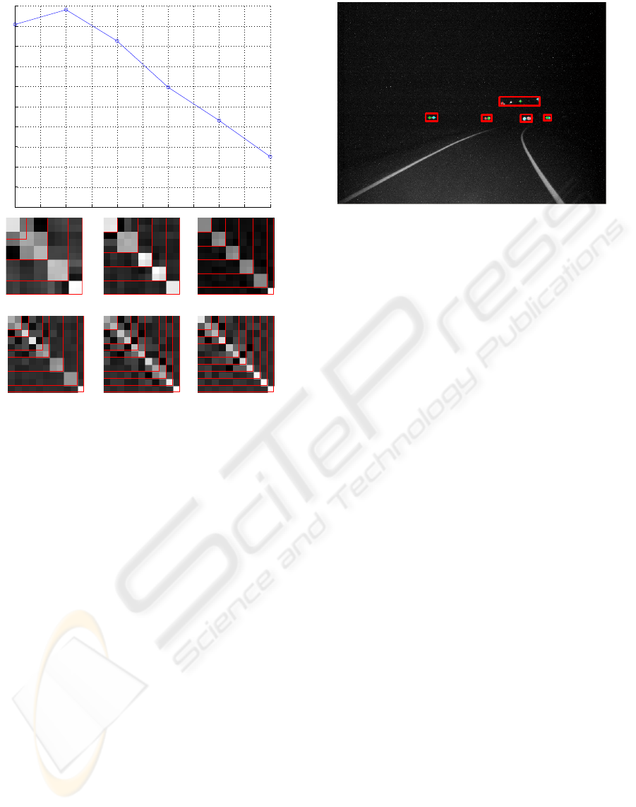
to find out possible block limits. Figure 1 shows an
example of rank r determination for the sequence 3.
Note that for r = 5 the block–diagonal aspect of the
computed Q
∗
is maximum. In fact, r = 5 provides
the right motion segmentation: the second 3×3 block
corresponds to three lamp posts, and each of the other
blocks is made of a couple of features which belong
to the same vehicle.
Let be l
1
,l
2
...l
r
the list of computed possible block
limits taken as those columns of Q
∗
r
= V
∗
r
V
∗t
r
where ε
shows a sharp increase. According to equation (5), a
normalized blockiness measure is defined as:
b(r)=
1
r
r
∑
k=2
sign(l
k
− l
k−1
− 1)( ε (l
k
) − ε (l
k−1
))
(14)
We select the right r as the one for which the
normalized energy within all the possible computed
blocks is maximum. However, blocks of size 1 fea-
ture are not taken into account, because for r = m, Q
∗
m
is perfectly diagonal with 1×1 blocks and we do not
want to interpret this situation as a case of maximum
blockiness. Figure 1 (top) shows an example of the
blockiness measure of Q
∗
r
for the possible values of r
according to equation (13).
Regarding strategy 1, the blocks for the best r yield
the motion segmentation. As for strategy 2, we use
the value of the blockiness measure to make a deci-
sion concerning the existence of more than one block.
A simple threshold (set at 0.7) can differentiate the
two cases in our experiments. In figure 2 the obtained
motion segmentation is shown.
4.2 3D Velocity Computation
The Han-Kanade (Han and Kanade, 2004) algorithm
allows to recover the velocity ratios of the features,
i.e. v
k
/v
l
 for each k,l = 1 ... m. The veloc-
ity values are useful not only to group the features
in objects but to distinguish between the objects that
are approaching and the ones that are moving farther
away from the camera, since their velocities have op-
posite sign.
The problem is that we would need to know which
of the points are static in order to obtain the real ve-
locity ratios, as it can be seen in section 3. But that
is, precisely, our final goal: to find out which of the
points correspond to vehicles and which to static fea-
tures (such as lamp posts or traffic signals).
The method described in section 3 solves the case
when the scene is 3D and the velocities of moving ob-
jects span a 3D space (rank(
ˆ
W)=6). Unfortunately,
degenerate cases can arise due to degenerate shape
and/or motion. Specifically, in the traffic sequences
we work with, the most common situation is the ex-
istence of one or multiple moving objects in the same
direction or perhaps opposite sense. As before, the
static structure of the objects is 3D, but 3D velocities
v
k
span only a one dimensional space, since they dif-
fer in module or sign but not in direction.
Therefore, we have to deal with a degenerate case
MOTION SEGMENTATION THROUGH FACTORIZATION - Application to Night Driving Assistance
273

4 4.5 5 5.5 6 6.5 7 7.5 8 8.5 9
0
0
.1
0
.2
0
.3
0
.4
0
.5
0
.6
0
.7
0
.8
0
.9
1
r = 4 r = 5 r = 6
r = 7 r = 8 r = 9
Figure 1: Sequence with m = 11 trajectories manually
tracked over n = 28 frames, showing four cars and three
lamp posts. Top : Measure of blockiness, sum of the nor-
malized energy of Q
∗
within the possible blocks larger than
1×1 features. The maximum is attained at r = 5. Bot-
tom: computed Q
∗
for r = 4...9.
in which rank(
ˆ
W)=4 and the motion and shape ma-
trices are:
M
2n×4
=
⎡
⎢
⎢
⎢
⎢
⎢
⎢
⎢
⎢
⎢
⎢
⎢
⎣
i
1
i
x1
i
2
2i
x2
.
.
.
.
.
.
i
n
ni
xn
j
1
j
x1
j
2
2j
x2
.
.
.
.
.
.
j
n
nj
yn
⎤
⎥
⎥
⎥
⎥
⎥
⎥
⎥
⎥
⎥
⎥
⎥
⎦
(15)
S
4×2n
=

s
1
s
2
... s
m
v
x1
v
x2
... v
xm

(16)
There is a rank-4 variant of the linear motion fac-
torization, through which we can compute S .Now,
we try to group features which share a similar veloc-
ity module: v
xj
.
First, we run the Han-Kanade algorithm and obtain
the velocities of the feature points: v
xj
. In fact, only
the ratios between the velocities are meaningful, not
Figure 2: Motion segmentation, sequence 3, Costeira-
Kanade method.
the actual value. Unfortunately, we can only recover
the real ratios in case we know which are the sta-
tic points and we subtract previously their velocity to
the vector v
xj
. Thus, we secondly compute the ratios
v
xk
/v
xl
for all pairs of features (k,l) and put them into
a matrix R. For pairs of features corresponding to the
same object (or at least, those that move in the same
way), a ratio near to 1 is obtained, since their veloc-
ity values are similar. We have experimentally fixed a
tolerance of tol = 0.3 and if we define q
kl
= v
xk
/v
xl
,
we change the matrix of ratios according to:
R
m×m
(k, l)=

q
kl
if |q
kl
−tol|≤1 ,
0 otherwise
(17)
The aim is to obtain a matrix whose non-zero el-
ements give us the motion segmentation. In the best
case, we obtain columns with at least 2 non-zero ele-
ments when the feature points correspond to a vehicle.
And for the static points, we obtain columns of one or
more non-zero elements.
For instance, taking again the sequence 3, we con-
struct the matrix of the ratios between the velocities R
(figure 3) and it results in the motion segmentation we
can see in figure 4. There are three 2× 2 blocks, that
correspond to three of the vehicles. The third 2 × 2
block (the third vehicle) and the last 3 × 3 (the three
lamp posts) are considered as a unique block. Thus,
there are 4 different motions. This is due to the similar
value of the velocity of one of the cars and the static
points. As we mention before, the correct segmenta-
tion would be obtained subtracting the velocity of the
static points. However, that is not possible, since we
can not know which of the points are the static ones.
VISAPP 2006 - MOTION, TRACKING AND STEREO VISION
274

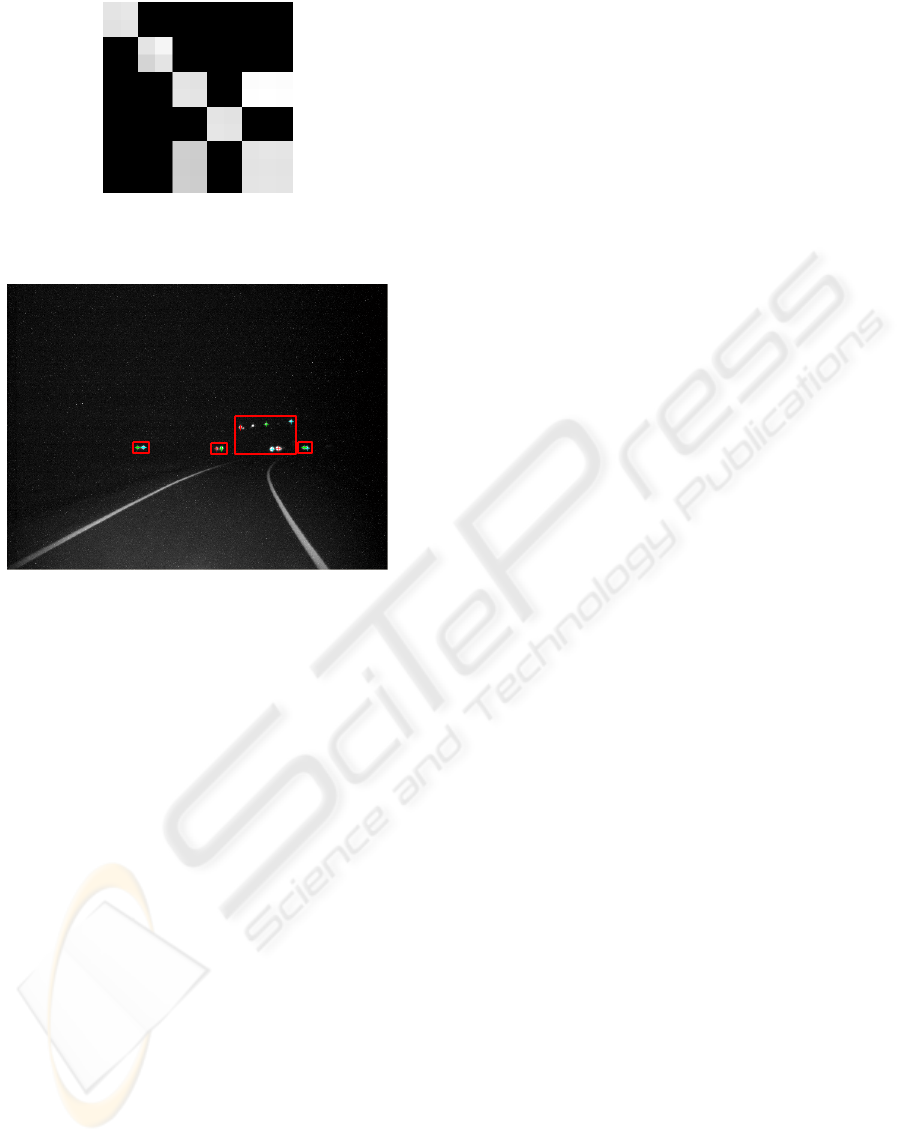
Figure 3: Matrix R of velocities ratios, Han-Kanade
method.
Figure 4: Motion segmentation for sequence 3, Han-
Kanade method.
5 RESULTS
We have tested both methods on 19 sequences ranging
from 9 to 30 frames, at a frame rate of 10 frames per
second. With these numbers, even oncoming vehicles
stay in the desired mid to far range distance. All fea-
tures are manually tracked to avoid gaps and errors in
the trajectories. Working with a tracker it would be
necessary to deal with occlusions, which is an addi-
tional problem not tackled in this paper. Additionally
the assumption that every vehicle appears at least as
two blobs could not be introduced. Hence, computa-
tional cost is added to the algorithm, since the range
of possible ranks ofW is extended (see inequality (13)
in section 4.1).
Table 1 summarizes the characteristics of the se-
quences and the obtained results for the vehicle ex-
istence test (when two or more feature groups are de-
tected, the answer is yes, otherwise we can not decide)
and motion segmentation, and for both methods. We
classify as good results the ones for which only few
mistakes are obtained or those that can be, in some
way, justified (for the characteristics of the sequence,
the features position or movement, etc). Figures 5-
7 show some examples of motion segmentation ob-
tained with both methods.
For the case of Costeira-Kanade adaptation, motion
segmentation fails in 8 out of 11 cases, where both
static and moving features are assigned to the same
group. But in two of them (sequences 5 and 6) the
vehicle is so far away that it can not exhibit a different
image motion regarding static points, also quite far
away. However, vehicle existence fails only in 4 and
can not decide in 2.
In the Han-Kanade adaptation, the results are bet-
ter when the feature points are far from the camera or
situated in the center of the image. This is necessary
to achieve a good approximation of the perspective
projection by an affine one. Besides, for this tech-
nique, it is important that the camera rotates. The ve-
hicle existence, however, provides better results. In
some cases, the velocities of features corresponding
to the same object have opposite sign and our al-
gorithm considers those features independent, so the
motion segmentation is not achieved. In most cases,
this problem would be solved subtracting the veloc-
ity of static points. Unfortunately, that information is
not available, since at the moment it is impossible to
distinguish between static and dynamic features.
6 CONCLUSION
In this paper we have addressed the problem of ve-
hicle detection at night when they are far away or at
a mid-range distance by adapting two different factor-
ization algorithms. The first one is due to Costeira and
Kanade and the second one to Han and Kanade. The
Costeira–Kanade method gives better results in the
motion segmentation. Besides, fewer feature points
are necessary. However, the method of Han–Kanade
is interesting because the matrix of trajectories does
not need to be sort like in the previous approach.
Moreover, it provides the ratios of the velocities of the
feature points. The problem is that we would need to
know at least one static point in order to have the real
velocity ratios.
One of the main problems we have to deal with is
the approximation of the perspective projection by an
affine one. It is quite difficult to find a sequence where
the points are far away (there the approximation is
better) and at the same time they have enough image
motion (then the factorization performs well).
In summary, the test of vehicle existence performs
fairly well for both of the methods, whereas right mo-
tion segmentation is more difficult to achieve. In the
future, the combination of the two factorization tech-
niques we have explored could be useful. We also
plan to work with longer sequences and address to the
problem of incomplete trajectories.
MOTION SEGMENTATION THROUGH FACTORIZATION - Application to Night Driving Assistance
275

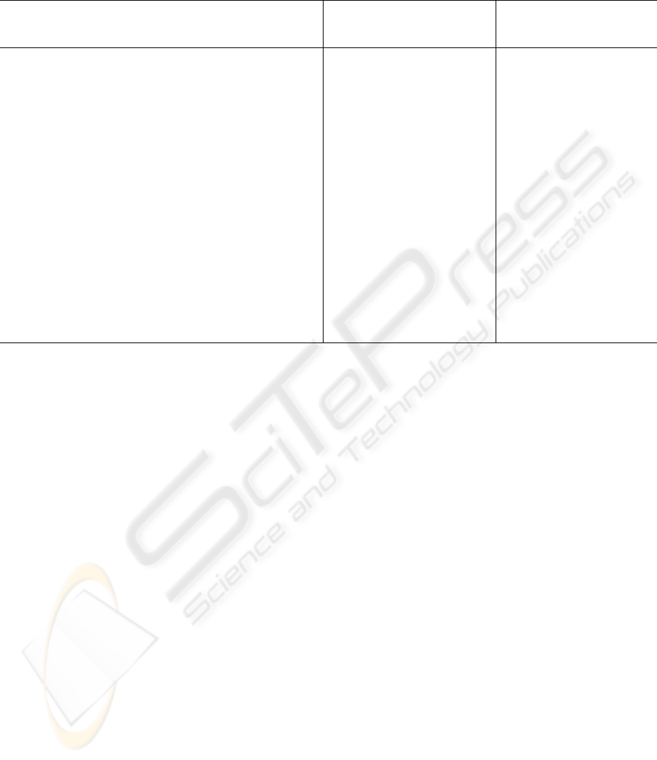
Table 1: Table of results for both methods.
Number Number Tracked Tracked Costeira–Kanade Han–Kanade
Sequence of of static
Vehicle Motion Vehicle Motion
frames features vehicles features
existence segmentation existence segmentation
1161042right right right fail
224822
right good right good
3281143
right right right good
4307Any7
don’t know right fail fail
524412
fail fail not tested
69413
fail fail not tested
7335Any5
don’t know right not tested
813832
fail fail right fail
913832
right right right good
10 12 8 1 6
fail fail right fail
11 14 10 3 4
right fail right good
12 26 9 3 3
not tested right fail
13 27 8 2 4
not tested right good
14 10 7 3 1
not tested right good
15 21 16 3 10
right fail right fail
16 20 14 3 8
right fail right fail
17 20 14 4 2
right fail not tested
18 21 7 2 3
right good not tested
19 19 10 2 6
right good right good
REFERENCES
Costeira, J. and Kanade, T. (1998). A multibody factoriza-
tion method for independently moving objects. Inter-
national Journal of Computer Vision, 29(3).
Han, M. and Kanade, T. (2004). Reconstruction of a scene
with multiple linearly moving objects. International
Journal of Computer Vision, 59(3):285–300.
Hu, U. (1999). Moving objects detection from time-varied
background: an application on camera 3d motion
analysis. Second International conference of 3-D dig-
ital imaging and modeling.
Kanatani, K. and Sugaya, Y. (2004). Factorization without
factorization : complete recipe. Memoirs of the Fac-
ulty of Engineering, Okayama University, 38(2):61–
72.
Megret, R. and DeMenthon, D. (2002). A survey of
spatio–temporal grouping techniques. Technical Re-
port LAMP–094, Language and Media Processing,
University of Maryland.
Tomasi, C. and Kanade, T. (1992). Shape from motion from
image streams under orthography : a factorization ap-
proach. International Journal of Computer Vision,
2(9).
Woelk, Gehrig, K. (2004). A monocular image based in-
tersection assistant. IEEE Intelligent Vehicles Sympo-
sium.
VISAPP 2006 - MOTION, TRACKING AND STEREO VISION
276

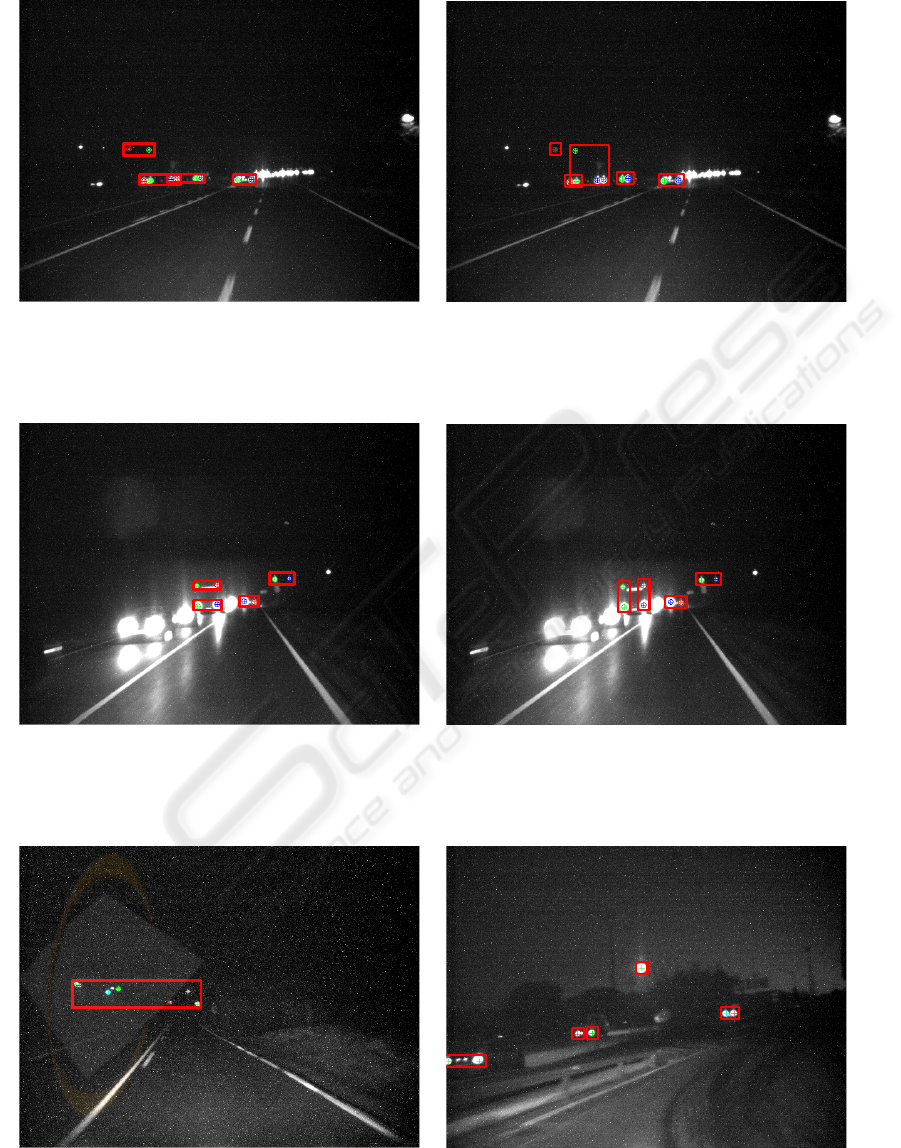
Figure 5: Sequence 1: four cars (three approaching the camera, one in the same direction) and two lamp posts. Left: Costeira–
Kanade method, the three cars of the left are considered a unique object. Right: Han–Kanade method, one lamp post is
grouped with one of the cars.
Figure 6: Sequence 2: one bus approaching the camera (four feature points), one car in the same direction as the camera and
two lamp posts. Left: Costeira–Kanade method. Right: Han–Kanade method. In both methods the features of the bus are not
grouped as a unique object, due to the perspective effect (in the last frames the bus is very close to the camera).
Figure 7: Left: Costeira–Kanade method. Sequence 4: seven static points, segmented as one object. Right: Han–Kanade
method. Sequence 14: three cars in the same direction as the camera and one lamp post. The features of the second car are
segmented separately.
MOTION SEGMENTATION THROUGH FACTORIZATION - Application to Night Driving Assistance
277