LOCAL KERNEL COLOR HISTOGRAMS FOR BACKGROUND
SUBTRACTION
Philippe Noriega, Benedicte Bascle, Olivier Bernier
France Telecom, Recherche & Developpement
2, av. Pierre Marzin, 22300 Lannion, France
Keywords:
Histograms, background subtraction, color quantization.
Abstract:
In addition to being invariant to image rotation and translation, histograms have the advantage of being easy
to compute. These advantages make histograms very popular in computer vision. However, without data
quantization to reduce size, histograms are generally not suitable for realtime applications. Moreover, they
are sensitive to quantization errors and lack any spatial information. This paper presents a way to keep the
advantages of histograms avoiding their inherent drawbacks using local kernel histograms. This approach is
tested for background subtraction using indoor and outdoor sequences.
1 INTRODUCTION
A normalized color histogram is easy to compute
and is invariant to rotation and translation of im-
age content. It is robust regarding partial occlusions
of objects of interest in the scene. These advan-
tages explain why histograms are widely used in com-
puter vision. Examples of applications are: content
based image retrieval (CBIR) (Han and Ma, 2002;
Pass and Zabih, 1996; H. Yamamoto and Takemura,
1999), tracking (B. Han and Davis, 2005; M. Ma-
son, 2001), background subtraction (A. Elgammal
and Davis, 2000; K. Toyama and Meyers, 1999)...
However, histograms have some drawbacks. First,
they lack any spatial information: two images can
have the same histogram and be dissimilar due to a
different ordering of the pixels in the images. A sec-
ond drawback occurs when histogrammed data is in-
sufficiently quantized. This problem generally im-
plies large histograms (several thousands of bins) re-
quiring important computation costs and preventing
real-time computation. Histograms are also sensi-
tive to image noise and to quantization errors that
may cause bin changes even though image variation
is small. So, bin by bin comparison measure can lead
to important dissimilarities between histograms from
similar pictures.
The goal of local kernel histograms is to deal with
these drawbacks while keeping the advantages of his-
tograms. This technique is applied on background
subtraction using local kernel color histograms to
demonstrate its efficiency. The next section presents
the related works, section 3 describes the local ker-
nel histograms taking example on color feature ex-
traction, section 4 explains how to apply them to
background subtraction, experimental results are pre-
sented in section 5 and section 6 concludes this paper.
2 RELATED WORKS
Some histogram techniques permit to recover miss-
ing spatial information. The color cooccurrence his-
togram (Chang and Krumm, 1999; Huang et al.,
1997) is an elegant solution where a histogram bin
b is associated with two colors c
1
, c
2
and a distance
d. The histogram bin b(c
1
, c
2
, d) records the number
of (c
1
, c
2
) colored pixel pairs wich are d distant. A
variant consist in only considering pixels belonging
to contours (Crandall and Luo, 2004). Color cooc-
currence histograms tend to have a huge number of
bins making real time computation difficult. Another
solution is to split the histogram bins in two classes
to classify coherent and incoherent pixels of the same
color (Pass and Zabih, 1996). A pixel is considered as
coherent if it is part of a homogeneously colored zone.
Otherwise, the pixel is considered as incoherent. This
method needs clustering algorithms to define the ho-
mogeneous zones. A last solution for this problem
consists in dividing the image in regions and comput-
213
Noriega P., Bascle B. and Bernier O. (2006).
LOCAL KERNEL COLOR HISTOGRAMS FOR BACKGROUND SUBTRACTION.
In Proceedings of the First International Conference on Computer Vision Theory and Applications, pages 213-219
DOI: 10.5220/0001363302130219
Copyright
c
 SciTePress

ing a histogram for each one. Each histogram is asso-
ciated with a local zone in the image providing spatial
information. A variant consists in dividing the im-
age in equal squares and compute one histogram for
each square (M. Mason, 2001). The Multi-Scale His-
togram Intersection Representation (MSHIR) (Gargi
and Kasturi, 1999) is another variant. It is a global to
local representation where the image is divided into
decreasing scale blocks. Another similar approach
consists in recursively dividing the image into regions
until each region has a homogeneous feature distribu-
tion or until the size of each region becomes smaller
than a given threshold value (H. Yamamoto and Take-
mura, 1999).
To reach real-time performance, it is necessary to
reduce the amount of data by quantizing the fea-
ture space before histogram computation. Consider-
ing color histograms, quantization consists in putting
close colors in the same histogram bin. Quantization
can be performed in different color spaces. (M. Ma-
son, 2001) applies a color depth reduction formula
to transform the 24-bit RGB color space to 12-bit,
(Crandall and Luo, 2004) work in CIE LAB color
space and reduce it to 267 standard colors in a first
stage before keeping only 10 basic colors. The CIE
LAB space has the advantage of being perceptually
uniform i.e. the Euclidean distance between two
colors corresponds to the human perception differ-
ence. The calculation of the distance between two
histograms is another way to reach real time com-
putation. In the case of quadratic histogram distance
(J. L. Hafner and Niblack, 1995), the weight matrix
that contains the coefficients denoting the similarity
between histogram bins can be diagonalized offline.
Filling several histogram bins with a unique pixel
is a good method to reduce influence of noise and
of quantization errors in histogram computation (Han
and Ma, 2002). Quadratic distance (J. L. Hafner and
Niblack, 1995) yields the same advantage but use
only the Euclidean distance in histogram similarity
computation.
3 COLOR LOCAL KERNEL
HISTOGRAMS
In the proposed technique, image is segmented into
overlapped local squares with a histogram for each
one to provide accurate spatial information. To re-
duce significantly the amount of data without loosing
important information because of coarse quantization,
the color space is quantized according to the most rep-
resentative colors extracted from the scene. A double
Gaussian kernel, one in the image space and one in
the color space bring robustness against noise. Tech-
nical implementation is described further below.
3.1 Image Partitioning
Histograms must be computed from a group of pix-
els. For maximum spatial accuracy, the image is par-
titioned in n × n square like regions that are over-
lapped with the same gap g for both image axis co-
ordinates. So, excluding the image edges, a pixel be-
longs to N
a
= (n/g)
2
regions.
On one hand, n must be large enough to smooth
both camera vibrations and waving objects in the
scene. On the other hand, too large regions prevent
accurate objects of interest detection. In experimental
results, n is fixed at 12 pixels with a gap g = 3. More
overlapping requires excessive computing resources.
3.2 Color Quantization
Quantization allows saving computer resources by re-
ducing the histogram sizes. Because camera noise
prevents distinguishing between all the 256×256 col-
ors in the U V space, this last is reduced to 40 × 40
colors. Then, a good option is quantizing taking into
account the most representative colors in the scene.
In this way, n
c
colors are selected from the image
reference to be associated to n
c
histogram bins. An
undefined color bin is added for other unselected col-
ors. Thus, all pixels not corresponding to one of the
selected colors is associated with the undefined color
bin.
This approach brings a great improvement in term
of computation time. To represent more than ninety
percent of reduced colors in a cluttered scene, the
color histogram size is set to only 15 color bins.
Moreover, this size is smaller than those reached
by good quantization: 64 with fuzzy histograms in
CBIR application (Han and Ma, 2002) or 1600 bins in
CIELAB (Crandall and Luo, 2004), and much smaller
than those usually reached: 4096 for the tracking al-
gorithm presented in (M. Mason, 2001) or 9796 for
color cooccurrence histograms (Chang and Krumm,
1999).
3.3 Kernels
Instead of associating one pixel with a unique region
and a unique histogram bin, Gaussian kernels are in-
troduced in both image and color space to bring more
flexible fuzzy associations between image and his-
tograms. Gaussian kernels are also chosen because of
its smoothing properties and are easily computed. For
computation efficiency, the kernels are pre-computed
and stored in lookup tables.
3.3.1 Spatial Gaussian Kernel
Pixels S
k
(x
k
, y
k
) in a local area l are weighted in
terms of distance from the area center. Thus, to com-
VISAPP 2006 - IMAGE ANALYSIS
214

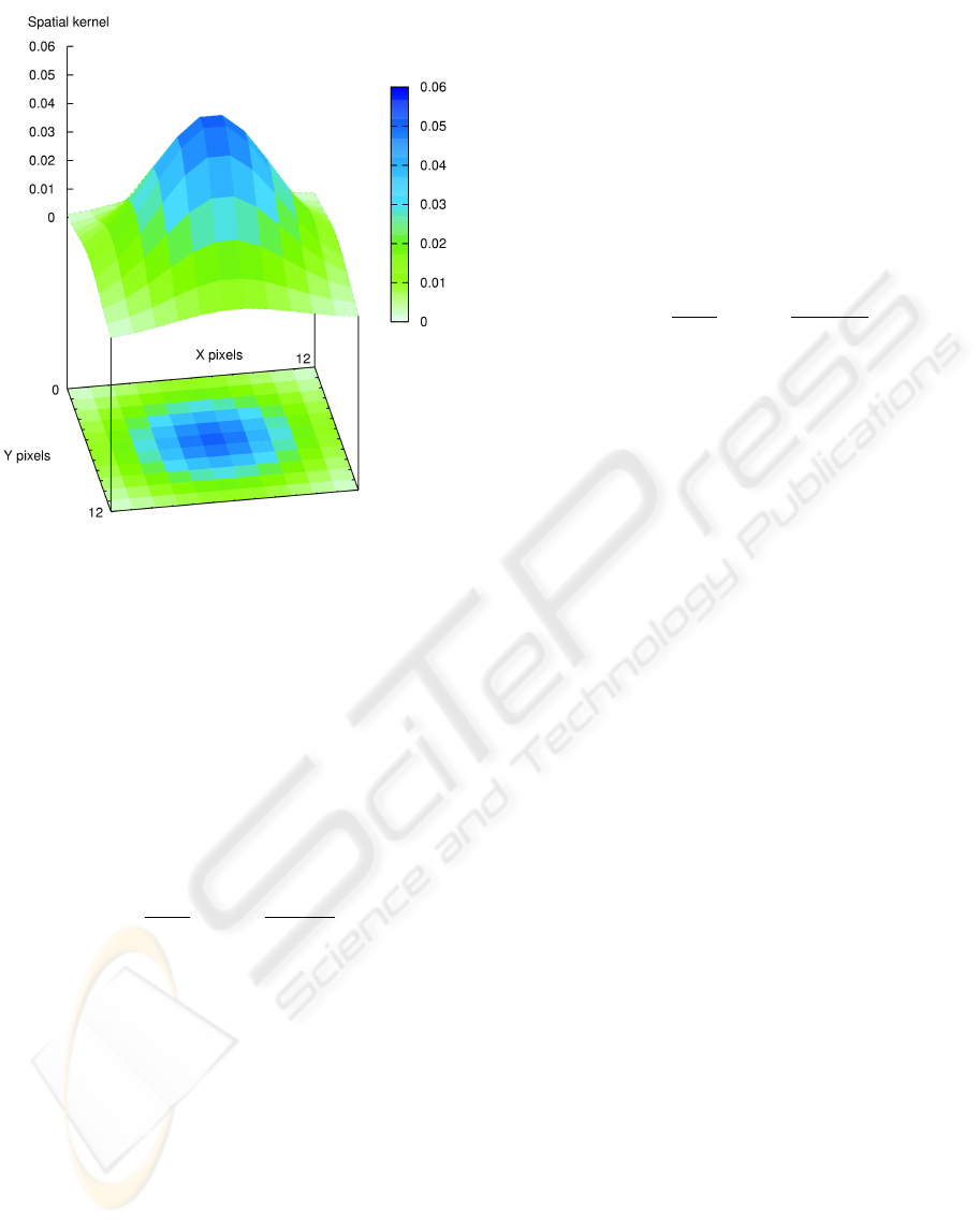
Figure 1: Spatial Gaussian kernel on a local area of 12 × 12
pixels. The standard deviation is low enough (σ
s
= 3) to
provide good smoothing properties.
pute the local histogram H
l
, the pixel contributions
are weighted according to a bi-dimensional spatial
Gaussian kernel G
S
l
(µ
S
l
, σ
s
) with mean µ
S
l
(x
l
, y
l
) on
the area center and standard deviation σ
s
(see Figure
1). K
S
is a normalization coefficient:
d
x
= x
k
− x
l
,
d
y
= y
k
− y
l
,
G
S
l
(S
k
) =
K
S
2πσ
s
exp −
d
2
x
+ d
2
y
2σ
2
s
!
.
(1)
The ratio weight between the border and center
area of regions must be low enough to provide good
smoothing properties. Thus, the standard deviation
σ
s
is chosen to be about a quarter of the local area
size. This setting brings 95 percent of the Gaussian
kernel inside the area and gives a ratio weight of
about 0.135. K
S
normalizes the kernel on the area:
P
n
2
k=1
G
S
l
(S
k
) = 1.
3.3.2 Color Gaussian Kernel
Two different colors falling in two separate histogram
bins are considered dissimilar even if they are very
close. This is a significant classical histogram draw-
back.
Using a color Gaussian kernel alleviates this prob-
lem and takes into account colors similarity. In-
stead of falling into a unique histogram bin, a
pixel is shared between several bins according to
a Gaussian weight G
C
. In Y UV color space and
given h
j
, a bin representing the color (U
j
, V
j
) in the
chrominance histogram, the contribution of the pixel
S
k
(x
k
, y
k
, Y
k
, U
k
, V
k
) to the h
j
bin is:
d
U
= U
k
− U
j
,
d
V
= V
k
− V
j
,
G
C
j
(U
k
, V
k
) =
K
C
j
2πσ
c
exp

−
d
2
U
+ d
2
V
2σ
2
c

.
(2)
K
C
j
is a normalization coefficient determined for
the color (U
j
, V
j
) among the n
r
colors in the reduced
space:
P
n
r
i=1
G
C
j
(U
i
, V
i
) = 1. Standard deviation σ
c
is estimated by taking into account the camera noise.
3.4 Local Kernel Histograms
Computation
As explained above, local kernel histograms are com-
puted from image overlapped regions taking into ac-
count the two Gaussian kernels: the former in image
space and the second in color space.
In a local area l, the value of a h
j
histogram bin
corresponding to a selected color (1 ≤ j ≤ n
c
) is:
h
j
=
n
2
X
k=1
G
S
l
(S
k
)G
C
j
(S
k
) . (3)
For the undefined color bin, all occurs as if his-
togram contains all the n
r
colors in the reduced space
(1 ≤ j ≤ n
r
). Then, the value of the undefined color
bin is the sum of unselected color bins:
h
j+1
=
n
r
X
(j=n
c
+1)
h
j
. (4)
Of course, for fast histogram computation, contri-
butions of each colors in the reduced color space are
pre-computed in lookups tables. The normalized his-
togram H
l
contains n
c
colors bins plus the undefined
color bin. It is normalized due to the normalization
constants K
C
and K
S
.
4 APPLICATION TO
BACKGROUND SUBTRACTION
In background subtraction, histograms are often used
to extract spatial or temporal features of background.
LOCAL KERNEL COLOR HISTOGRAMS FOR BACKGROUND SUBTRACTION
215

Those can being color or contours orientation for spa-
tial features or pixel value versus frame number in
the case of temporal features. For example (A. El-
gammal and Davis, 2000) compute their background
model using histograms that describe temporal statis-
tics for pixels values. In their region scale process,
(K. Toyama and Meyers, 1999) use histograms to
compare moving regions between frames. This sec-
tion describes how to apply local kernel histograms in
color background subtraction to obtain a pixel scale
probability map.
4.1 Local Area Probability
As histograms are normalized, the Bhattacharyya dis-
tance between them provides a result between 0 and
1 which can be assimilated as a probability. Given
histograms H
t
0
l
and H
t
l
computed from the same
area l respectively in reference and current image,
the probability P
l
that l belongs to the background
is computed applying Bhattacharyya distance to the
histogram bins h
j
.
P
l
=
n
c
+1
X
j=1
q
h
t
0
j
h
t
j
. (5)
4.2 Pixel Probability
Area histogram similarity computation provide an
identical probability for all the pixels in the area.
Thus, the resulting probability map is heavily aliased.
If it is suitable for tracking (M. Mason, 2001), back-
ground subtraction needs generally more spatial ac-
curacy. Overlapping between areas reduce aliasing
but there is a trade off between computation time and
gap size between areas. To provide a pixel scale map
while preserving computation ressources, the prob-
ability is computed with the probabilities resulting
from the N
a
areas that a pixel belongs to. Taking ac-
count of the spatial kernel G
S
, the probability P
s
for
the pixel S(x
k
, y
k
, Y
k
, U
k
, V
k
) is:
P
s
=
1
N
a
N
a
X
l=1
G
S
l
P
l
. (6)
5 EXPERIMENTAL RESULTS
The local kernel histograms are compared with three
other algorithms in the field of background subtrac-
tion. Each algorithm use chrominance channels U V
from Y UV color space:
Mean & Threshold: Pixel-wise mean values
are computed during a training phase, and pixels
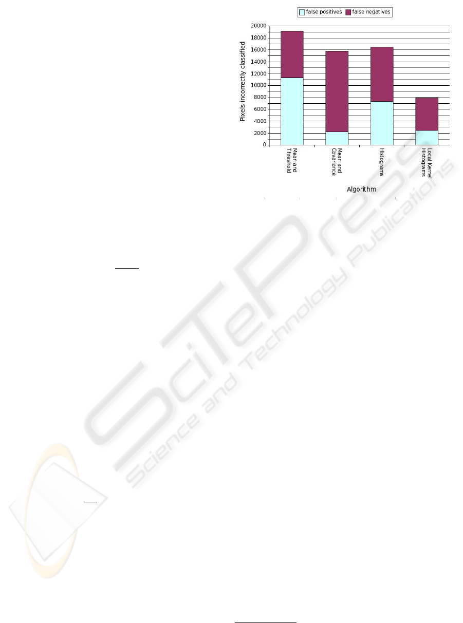
Figure 2: Algorithms overall performance.
within a fixed threshold of the mean are considered
background.
Mean & Covariance: The mean and covari-
ance are computed from the recent samples values
for pixels. Foreground pixels are determined using a
threshold. This is similar to the background algorithm
used in (A. Elgammal and Davis, 2000).
Histograms: Frames are segmented into 50%
large overlapped square zones of 20 pixels. A
conventional color histogram is computed from
each zone for both reference and current image.
Similarity is computed with histogram intersection
and a threshold determines foreground pixels: see
(M. Mason, 2001).
Local Kernel Histograms: The method explained in
this paper, probability map is thresholded to extract
silhouettes.
Both indoor and outdoor test sequences are used
(see Figure 3). The third (foreground covers monitor
pattern) and the fourth (waving trees) sequences were
used by (K. Toyama and Meyers, 1999). They are
available from the web
1
in color with a 160×120
pixels resolution. The first indoor scene was grabbed
with a color CCD camera using 384×288 pixels
resolution and the last outdoor scene with a webcam
and a 320×240 pixels resolution. Image quality is
relatively poor. The five sequences show classical
difficulties for background subtraction:
1
http://research.microsoft.com/users/jckrumm/
WallFlower/TestImages.htm
VISAPP 2006 - IMAGE ANALYSIS
216

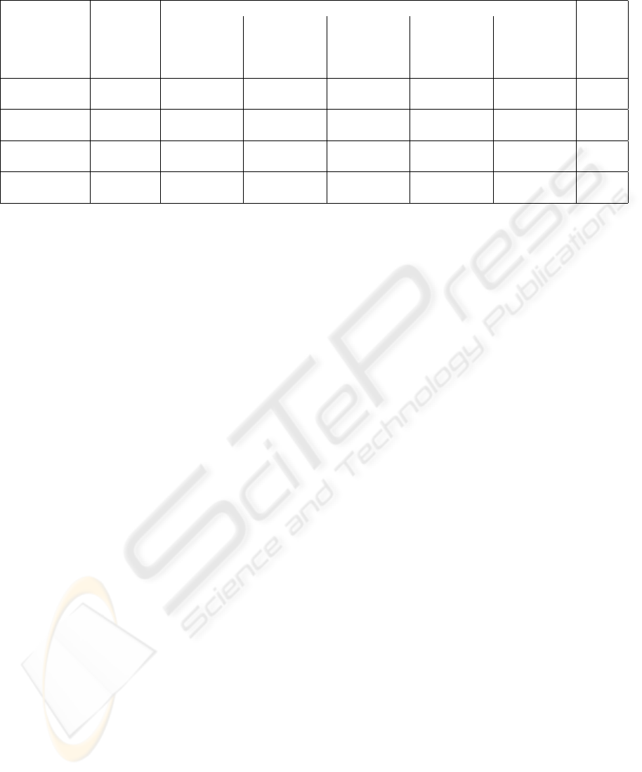
Table 1: Performance of algorithms on various images test.
Problem Type and his Associated Frame Test
Camera Indoor Foreground Waving Unexpected
Vibrations Covers Trees Gust of
Error Monitor Wind Total
Algorithm Type (frame 235) (frame 235) (frame 251) (frame 247) (frame 246) Errors
Mean and false neg. 0 6351 457 104 971
Threshold false pos. 2787 1848 195 1905 4554 19172
Mean and false neg. 0 6788 3273 977 2589
Covariance false pos. 49 603 89 116 1333 15817
Histograms false neg. 0 4525 2455 931 1207
false pos. 338 4507 32 96 2359 16450
Local Kernel false neg. 0 3247 664 195 1390
Histograms false pos. 0 692 146 495 1126 7955
Camera Vibrations: Camera is not strongly
fixed and vibrations cause small image motion.
Shadows and Reflections: A person stays be-
tween the window and the door. Shadow and
reflections slightly modify the background on the left
side of the picture.
Foreground Covers Monitor Pattern: A mon-
itor lies on a desk with rolling interference bars. A
person walks into the scene and occludes the monitor.
Waving trees: A person walks in front a sway-
ing tree.
Gust of Wind: A person walks in front of swaying
flowers. Suddenly, a gust of wind occurs. The flowers
move with more intensity.
The test images are shown in Figure 3. Tests are
performed on a single frame from each sequence and
consist in segmenting a human subject from the back-
ground. Mean & Threshold and Mean & Covariance
algorithms are both initialized during the first 200
frames before the test. Histogram based algorithms
are only trained with the first image of the test se-
quence.
Because histograms naturally have the capacity to
smooth noise, camera vibrations and swaying flowers
do not affect histogram based algorithms. If the Mean
and Covariance algorithm succeeds on the waving
trees scene, it needs a certain time to adapt its back-
ground model causing false detections when an unex-
pected event occurs e.g. a gust of wind. On the other
hand, conventional histograms fail when shadows and
reflections appear in the scene. In this case, U V
colors channels are slightly modified yielding pixels
jumps between histograms bins and obviously, con-
ventional histograms bin by bin comparison measures
fails. It is a classical histogram drawback. However,
small color changes do not affect local kernel his-
tograms because the color kernel reduces quantization
errors. Conventional histograms (M. Mason, 2001)
result in strongly aliased foreground detection. Thus,
because of their poor spatial accuracy, histograms are
generally not suitable for silhouette pose or gesture
analysis. However, local kernel histograms provide
spatial accurate probability maps (cf. § 4) for silhou-
ette extraction.
The results of the tests are shown in Figure 2 and
table 1. As in (K. Toyama and Meyers, 1999), per-
formances are evaluated in term of number of fore-
ground pixels marked as background (false negatives)
and background pixels marked as foreground (false
positives). Ground truth is provided by hand seg-
mentation. It is obvious that the few test sequences
produced in this paper are not sufficient to correctly
evaluate the difference between the algorithms. How-
ever, results underline the capacity of local kernel
histograms to naturally smooth noise from camera,
soften shadows or reflections and waving background
objects.
In terms of computation load, the local kernel his-
tograms modelizes a local area including n
2
pixels
with a histogram comprising n
c
+1 bins. In our exper-
iments, 144 pixel in a local area are modelized with
only 16 bins. Moreover, Gaussian kernels are pre-
computed and stored in lookup tables, yielding a fast
histogram computation. Thus, even with strong over-
lapping between local areas, computation times are
close to those required by the Mean & Threshold al-
gorithm.
6 CONCLUSION
As shown in experimental results, the local kernel
histogram based algorithm is a robust and efficient
LOCAL KERNEL COLOR HISTOGRAMS FOR BACKGROUND SUBTRACTION
217

method to extract color information from images.
Even in noisy environment with camera vibrations
or swaying vegetation, they provide useful and accu-
rate probability map for background subtraction. This
method is easily generalizable to other features e.g.
contours, and can be useful in many fields of com-
puter vision e.g. content based image retrieval (CBIR)
or tracking. This paper has demonstrated that local
kernel histograms combine conventional histograms
advantages and avoid their inherent drawbacks to pro-
vide robust, fast and accurate spatial information. Il-
lumination robust background subtraction using con-
tour features and local kernel histograms will be ad-
dressed in future works.
REFERENCES
A. Elgammal, D. H. and Davis, L. S. (2000). Non-
parametric model for backg round subtraction. In Eu-
ropean Conference on Computer Vision, volume II,
pages 751-767. Springer-Verlag.
B. Han, C. Yang, R. D. and Davis, L. (2005). Bayesian
filtering and integral image for visual tracking. In
Special session on Real-Time Object Tracking: Algo-
rithms and Evaluation in Workshop on Image Analysis
for Multimedia Interactive Services (WIAMIS).
Chang, P. and Krumm, J. (1999). Object recognition with
color cooccurrence histograms. In IEEE Conference
on Computer Vision and Pattern Recognition. IEEE
Computer Society.
Crandall, D. and Luo, J. (2004). Robust color object detec-
tion using spatial-color joint probability functions. In
IEEE Computer Society Conference on Computer Vi-
sion and Pattern Recognition (CVPR’04 ) - Volume 1,
pp 379-385. IEEE Computer Society.
Gargi, U. and Kasturi, R. (1999). Image database query-
ing using a multiscale localized color representation.
In IEEE Workshop on ContentBased Access of Image
and Video Libraries. IEEE Computer Society.
H. Yamamoto, H. Iwasa, N. Y. and Takemura, H. (1999).
Content-based similarity retrieval of images based
on spatial color distribution. In Int. Conf. on Im-
age Analysis and Processing (ICIAP), pp. 951-956.
Springer.
Han, J. and Ma, K. K. (2002). Fuzzy color histogram and its
use in color image retrieval. In IEEE Transactions on
Image Processing, vol. 11, no. 8, pp. 944-952. IEEE
Computer Society.
Huang, J., Kumar, S., Mitra, M., Zhu, W., and Zabih, R.
(1997). Image indexing using color correlograms. In
Proc. IEEE Comp. Soc. Conf. Comp. Vis. and Patt.
Rec., pages 762-768. IEEE Computer Society.
J. L. Hafner, H. S. Sawhney, W. E. M. F. and Niblack,
W. (1995). Efficient color histogram indexing for
quadratic form distance functions. In IEEE Trans-
actions. Pattern Anal. Mach. Intell. 17(7): 729-736.
IEEE Computer Society.
K. Toyama, J. Krumm, B. B. and Meyers, B. (1999). Wall-
flower: principles and practice of background mainte-
nance. In ICCV, pages 255-261. IEEE Computer So-
ciety.
M. Mason, Z. D. (2001). Using histograms to detect and
track objects in color video. In 30th AIPR Workshop.
pp. 154-159. IEEE Computer Society.
Pass, G. and Zabih, R. (1996). Histogram refinement for
content-based image retrieval. In IEEE Workshop on
Applications of Computer Vision. IEEE Computer So-
ciety.
VISAPP 2006 - IMAGE ANALYSIS
218

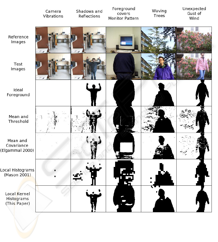
Figure 3: Comparison of color background subtraction algorithms with color local kernel histograms. The top row shows
reference images used to initialize background subtraction. The second row corresponds to original images extracted from
indoor and outdoor scenes. Third row represents hand segmented ground truth. Each other row shows the result for one
algorithm and each column represents a conventional problem.
LOCAL KERNEL COLOR HISTOGRAMS FOR BACKGROUND SUBTRACTION
219