LOCAL MINIMUM DISTANCE FOR THE DENSE DISPARITY

ESTIMATION

Eric Alvernhe

EMA, Lgi2p

ımes, France

* Philippe Montesinos, *Stefan Janaqi,† Min Tang

*EMA Lgi2p,+Nanjing university of science and technology

ımes France, †Nanjing China

eywords:

Stereo, Dense disparity map, Partial derivative equations, minimum distance.

Abstract:

This paper presents a new algorithm to solve the problem of dense disparity map estimation in stereo-vision.

Our method is an iterative process inspired by variationnal approach. A new criteria is used as the attachment

term based on the distance to local minimum of a similarity measure. Our iterative process is heuristic. Nev-

ertheless, we are able to interpret this algorithm presenting both combinatorial and continuous characteristics.

The quality and precision of the results obtained by our method both on image benchmarks and real data

clearly demonstrate the the validity of this approach.

1 INTRODUCTION

The aim of stereo-vision is to give a perception of a

scene in three dimensions using two or several im-

ages taken from different points of view. Usually,

stereo-vision is used to compute three dimensions re-

construction of rigid scenes. In order to solve this

problem, we need ﬁrst to compute matches between

features of the given images. This paper focuses on

stereo-vision image matching.

Matching problem often appears in various vision

tasks such as: motion, image registration, pattern

recognition, and stereo-vision. Unfortunately, each

similarity measure that can be deﬁned gives a percent-

age of false matching due to noise and ambiguity. In

sparse stereo matching, we often concentrate on fea-

tures or image primitives such as points of interest,

segments, regions. As an example, points of inter-

est (Gouet et al., 1998) are especially chosen for their

neighborhood speciﬁcity to reduce matching ambigu-

ity (points of interest are frequently used to recover

the epipolar geometry in uncalibrated stereo-vision).

Generally a matching scheme proceed in two steps,

a ﬁrst step of computing scores of similarity and a

second step of relaxation involving geometrical infor-

mations able to deal with ambiguous and weak corre-

spondances.

In this paper, we are interested in dense correspon-

dences i.e correspondences of all non occluded pix-

els of the image. The matching of image features

have obtained a lot of attention in the literature see

(Scharstein et al., 2001). The results of all these meth-

ods can be compared on the basis of the disparity

maps that they can deliver. Roughly speaking, dis-

parity is a value related to the displacement of pixels

from one image to another, and the disparity map con-

tains the disparity value of all the matching pixels (a

precise deﬁnition of disparity will be given in the next

section).

Different characteristics allow to give the speci-

ﬁcity of dense matching in comparison to the sparse

one:

• Disparity map is deﬁned over the entire image do-

main. It has to be a piecewise continuous function

preserving the edge’s depth.

• Concerning the improvement of the ambiguous

matches (as in textured region for example), relax-

ation cannot be done over the entire image domain

for obvious computational reasons. It is the role of

a global regularization constraint to overcome this

problem.

Features like segments or corners points (Boufama

and Jin, 2002) have been intensively studied for

stereo-vision but they cannot lead to precise dense

disparity maps, principally due to the fact that these

features do not appear on the homogeneous areas of

the images. The use of regions for matching is dif-

ﬁcult because of the lack of robustness of the char-

acterization of regions under projective transforma-

341

Alvernhe E., Montesinos P., Janaqi S. and Tang M. (2006).

LOCAL MINIMUM DISTANCE FOR THE DENSE DISPARITY ESTIMATION.

In Proceedings of the First International Conference on Computer Vision Theory and Applications, pages 341-348

DOI: 10.5220/0001369803410348

 SciTePress

tions. Dynamic programming often focuses on the

study of speciﬁc lines in the image (i.e the epipolar

lines presented in the next section) doing a combi-

natorial search for matches. This search has to sat-

isfy a regularity constraint on these lines and between

them (Ohta and Kanade, 1985). The satisfaction of

this constraint, while preserving edges, remains a dif-

ﬁcult task.

With the development of the Partial Derivative

Equations (PDE) and the increase of the computa-

tional speed, a new strategy based on a variational ap-

proach has been proposed by (Alvarez et al., 2000).

Their scheme naturally introduces a global regularity

constraint and a depth edge constraint into the varia-

tional formulation. After solving the Euler-Lagrange

equation they obtain a PDE composed of two terms: a

regularization term and an attachment term. As their

PDE is a gradient descent of an energy functional,

it is very important to have an energy “as convex as

possible”. For this reason, they use a coarse-to-ﬁne

approach based on a multi-scale gaussian smoothing,

and at each scale, they compute a disparity map. At

the end of this process they obtain the ﬁnal disparity

map.

Recently (Maier et al., 2003) has proposed a non

hierarchical approach which takes into account the

edges accurately. In (N.Slesareva et al., 2005) the

authors propose to use a Total Variation regularization

(Blomgren, 1998) and an attachment term coming

from the optical ﬂow literature. This method seems

to give promising results especially for noisy images.

We propose a new scheme allowing to compute di-

rectly the disparity map without multi-scale approach.

As the other methods our approach involves two terms

of regularity and data attachment. As regularity term,

we use the regularity constraint of (Alvarez et al.,

2000), but for the attachment term, in order to over-

come the problem of numerous local minima (one of

the characteristics of the dense matching), we use the

signed distance to the local minima given by a sim-

ilarity measure. With this modiﬁcation, our scheme

is no more deduced from a variational method but,

the iterative process that we have deﬁned has heuris-

tic justiﬁcations:

• All pixels minimizing a given similarity measure

are candidates for matching and have the same im-

portance. For the non ambiguous pixels, the match-

ing candidate is often unique and will be the ﬁrst

match found by our iterative process. For ambigu-

ous ones (as in textured region) the regularity con-

straint is used to improve the matches.

• Local minima of the similarity measure which are

close to each other collapse into one in the set

of matching candidates for our attachment term.

The resulting winning position is the one with the

Figure 1: Epipolar constraint: plane (P, C

) intersects

and l

and p

are projections of P on the images.

and p

lie on the epipolar lines.

smallest disparity measure.

Our regularisation term is continuous, while the at-

tachement term can be considered as combinatorial

by its discrete valuations. In the following of this pa-

per our method will be referenced as Iterative Scheme

to Local Minima (ISLM). Note that the combinatorial

aspect of our method is not implemented as a kind of

relaxation, but by properties of the valuation of our

attachment term.

The paper is organized as follows: section 2

presents the epipolar constraint and the disparity map.

Section 3 presents PDE based on variational approach

(Alvarez et al., 2000). The role of Nagel-Enkelmann

operator, used in our work, as a diffusion-reaction

term preserved discontinuity will be explained here.

Section 4 presents our attachment term and its prop-

erties, we discuss the differences with the Alvararez

variational approach. Our generic attachment term

can be computed with different similarity measures,

and we present here a simple square difference on

a correlation mask. Section 5 develops the compu-

tation of our attachment term. Finally, in section

6 experimentations are presented. We use synthetic

data where the true disparity is known and also real

images. The pertinence of our approach is demon-

strated by quantitative results when the true disparity

is known, and by qualitative results otherwise.

2 EPIPOLAR GEOMETRY AND

DISPARITY ESTIMATION

We note by I

and I

the two different views of a rigid

scene. Each three-dimensional point P of the scene

form a plane with the two optical centers C

and C

The intersection of this plane and the retinas are

lines, respectively l

and l

called epipolar lines. The

epipolar constraint expresses the fact that pixels p

and p

, which are respectively the projections of P on

and I

, lie respectively on l

and l

(see Figure (1)).

VISAPP 2006 - MOTION, TRACKING AND STEREO VISION

342

Lambda

Figure 2: λ is the signed distance from projection o of p

on epipolar line l

to p

In practice, the epipolar constraint allows the re-

duction of the search space for a corresponding pixel

of p

(image I

) to the line l

instead of all the im-

age domain I

. As a consequence, epipolar constraint

increases the matching quality and the computational

speed. This constraint is algebraically expressed by

the fundamental matrix 3 × 3 F .

We have:

, 1) =

) (1)

with

+ b

+ c

=0 (2)

where, p

, 1) and p

, 1) are

projective pixels coordinates,

) represents

the equation of l

. So, the epipolar constraint can be

written as:

, 1) F

, 1) = 0 (3)

In the following, we will consider that the funda-

mental matrix is known, (see for fundamental matrix

computation (Torr and Murray, 1997; Zhang et al.,

1994)).

We need to estimate the disparity of all the pixels.

Disparity for a pixel p

is a two dimensional afﬁne

vector h = p

in the image I

(keeping coordinates

of p

from the image I

). Thanks to the fundamental

matrix, only one coordinate of this vector needs to be

memorized. If we note o the projection of p

on l

we have h = p

o + op

with:

p

o =



+ b

(4)

Using the fundamental matrix, disparity h can be

deﬁned only by op

which will be referred as λ in

the following (see ﬁgure (2)). Thus, our dense stereo

correspondence problem is reduced to the estimation

of a grey level image λ over the image domain chosen

to be I

3 A VARIATIONAL APPROACH

FOR STEREO-VISION

This section presents the variational minimization ap-

proach introduced by (Alvarez et al., 2000) in order

to solve this stereo-vision problem. We explain there

the role of the Nagel-Enkelmann operator.

The functional energy E

var

model classically con-

tains two terms:

var

(λ)=CE

Regular

(∇λ)+E

Attach

(λ) (5)

In order to minimize this functional we can use a

gradient descent strategy after discretization with the

corresponding PDE:

dλ(t)

= −∇E

var

(λ(t)) (6)

We note here λ(t) the image obtained after t iter-

ations of the gradient descent. To obtain a good dis-

parity result with this PDE, two conditions must be

veriﬁed:

• The disparity image corresponding to the global

minimum of the energy must be close to the

true disparity one, the minimization of variational

method (eq. 5) is well designed to our stereo prob-

lem.

• The λ

tmax

solution obtained by the PDE (6) has to

be the global minimum of the variational function

(5).

To avoid local minima of their PDE, the authors

use a coarse-to-ﬁne hierarchical approach based on

gaussian smoothing, see (Alvarez et al., 2000) for

more details. Now we are going to discuss the ﬁrst

condition just stated before.

3.1 A Deﬁnition of Energy

We note Ω the entire image domain deﬁned with vari-

able x and y and

(x, y):=I((x, y)+h(λ))

The equation (eq. 5) is composed of two terms of

different weights C and 1.

The regularization term is deﬁned as follows:

Regular

Ω

|∇(I

+2ν

∇λD(∇I

) ∇λdxdy

(7)

with :

D(∇I





−

∂I

∂y

∂I

∂x





−

∂I

∂y

∂I

∂x



+ ν



(8)

The attachment term is:

Attach

(λ)=



Ω

(x, y)−I

(x, y))

dx dy (9)

The PDE obtained by the Euler-Lagrange condi-

tions from equation (5) is:

LOCAL MINIMUM DISTANCE FOR THE DENSE DISPARITY ESTIMATION

343

dλ



Ω

Cdiv(D(∇I)∇λ)+

(x, y) − I

(x, y))

∂I

∂y

+ b

∂I

∂x



+ b

dx dy

with reﬂecting boundary conditions.

The role of these two terms of the PDE in our stereo

problem is:

• The minimization of the attachment term implies

that the matches must have close intensity values,

according to a lambertian hypothesis.

• The minimization of regularization term imposes a

continuity constraint in the disparity image. In ho-

mogeneous regions the disparity should be contin-

uous with a step at the depth edges.

More details of the Nagel-Enkelmann reaction-

diffusion operator used for the regularization process

will be presented in the next subsection. The differ-

ent attachment terms will be discussed in detail in the

section 4.

3.2 Nagel-Enkelmann Operator

Nagel-Enkelmann operator has received a lot of

attention in computer vision, especially for optical

ﬂow analysis(Nagel, 1983). From a physical point

of view, it can represent the behavior of the heat

distribution in an isolated volume (with neglected

convexion). We give an example in the ﬁgure (3),

where we compute Nagel-Enkelmann diffusion in a

“Florence ﬂask”.

The initial heat distribution is given at the image

heat

and the ﬂask is associated to an image Flask.

Note that the heat diffusion is isotropic inside the

Florence ﬂask, and is stopped by reaction at the edge.

We will brieﬂy explain the equivalence between

this diffusion-reaction and our problem. Then we

will discuss the role of each element of the Nagel-

Enkelmann operator.

The heat(x, y), intensity value is the heat at the

point (x, y) corresponding to the disparity λ(x, y)

in our stereo problem, and I

plays the role of the

image Flask. When multiplying by ∇λ, the ﬁrst

term of equation (8) produces the reaction in the

PDE (diffusion direction is constraint to be along

the edge). The second term acts as a diffusion (into

the PDE it corresponds to a classical heat equation

in an homogeneous medium). ν is the weight of the

diffusion term. The equation (7) is normalized by

|∇(I

+2ν

Figure 3: Diffusion-Reaction with Nagel-Enkelmann Oper-

ator, ﬁrst and second image represent respectively the ﬂask

and the initial heat value (circle image) images 3 and 4 are

the diffusion-reaction after respectively 2000 and 5000 it-

erations, dt=0.3, total heat i.e sum of pixel’s intensities re-

mains constant.

In this scheme, diffusion will allow to extend the

disparity value in homogeneous regions (and so ex-

press regularity constraint), and the reaction term will

preserve depth contour. To preserve these depth con-

tour, we use the gradient of image I

, because a depth

edge implies an image edge. Note that an image edge

does not always correspond to a depth edge (for ex-

ample, the edges of the paving stones on the ﬂoor in

the image corridor (see ﬁg. 7)).

Next, we give an attachment term taking into ac-

count the similarity measure, especially for the am-

biguous matches.

4 TWO DIFFERENT

ATTACHMENT TERMS

This section presents our attachment term and how it

deals with ambiguous matches by embedding the dis-

tance to the local minima of a similarity measure. We

present ﬁrst the similarity measure used by Alvarez.

4.1 Attachment Term of the

Variational Approach

Under lambertian hypothesis the attachment term

used by Alvarez is expressed as the square difference

of grey levels:

(x, y) − I

(x, y)|

(10)

The main inconvenience with this formulation is

that it creates numerous local minima corresponding

to the possible disparities. As a consequence, these

local minima can easily drive the search of the dispar-

ity image toward a false solution. To overcome this

problem the authors have introduced a multi-scale

approach.

Local minima occur frequently in dense disparity

problems, and the similarity measure given by the

VISAPP 2006 - MOTION, TRACKING AND STEREO VISION

344

squared difference of intensities is not well-suited

to discriminate which local minima corresponds to

the true disparity. Moreover, even if it is natural in a

classical denoising image algorithm to use difference

of intensity pixels as attachment term, it will be

natural for the disparity map estimation to introduce

a difference of disparity as attachement term.

4.2 A New Attachment Term

Our attachment term is the following:

Attach



Ω

Disp

min

(x, y, λ)

dx dy (11)

where,

Disp

min

(x, y, λ) = argmin

d∈[−V,V ]

(S (I

(x, y),I

(x, y)

λ+d

))

(12)

with,

• S a similarity measure between the pixel at (x, y)

coordinates from image I

and the pixel (x, y)+

h(λ + d)) from image I

. S equals 0 if the pixels

are similar and otherwise a positive value .

• V is a ”small” integer constant. For a pixel (x, y) at

the current disparity λ, Disp

min

is the signed dis-

tance which can minimize the similarity measure in

the interval [−V, V ]

Our attachment cannot lead to a gradient strategy

from Euler-Lagrange as in variational method, be-

cause arg min is not a function. To minimize heuris-

tically this energy, we use the iterative process:

dλ

= Cdiv(D(∇I))∇λ + Disp

min

(x, y, λ)

Note that it is classical to lose the variational mean-

ing in regularization PDE techniques such as MCM,

AMSS regularization for example. Anyway, these

PDE have some good interpretations, because they are

deﬁned in the multi-scale frame (Alvarez et al., 1992;

Chambolle, 1994). They correspond to PDE deﬁned

by properties such as isotropy, euclidean invariance,

afﬁne invariance, etc. Due to the use of the arg min,

and because of the violation of comparison principle

(Alvarez et al., 1992), our iterative process is not de-

ﬁned in the multi-scale approach. Nevertheless, we

can deﬁne directly some good properties for this It-

erative Scheme to Local Minimum (ISLM). Iterative

processes using arg min have been used for classi-

ﬁcation problems (MacQueen, 1967). Here we have

to give at each pixel a value in a class, and it is the

purpose of the arg min. We can deﬁne some links

between our problem and a classifying one : the dif-

ferent class for a pixel with our method are the min-

ima of their similarity measure S.

Taking the signed distance to the local minima as

the attachment term gives four principal properties:

• The number of matching candidates is decreased

because local minima of the attachment term of

PDE that are near to each other collapse into one

for ISLM. The position of this minimum corre-

sponds to the one with smallest similarity. A mini-

mum for the d

min

attachment term corresponds to a

minimal similarity S in the neighborhood [−V,V ].

By the way, all local minima m

, ... for the

similarity measure S, employed by the PDE, with

d(m

) <V, collapse into one in ISLM. The

position of this minimum is the pixel correspond-

ing to the one with the smallest similarity measure.

Let m

be the minimum found by fusion of m

and

. After collapsing, the attraction interval domain

of m

will be [m

− V,m

+ d(m

)+V ] due

to the absorption of m

• Our attachment term gives the same weight to all

local remaining minima, and has no effect on ho-

mogeneous areas, so the regularization process can

move the disparity from a local minimum to an-

other one easily by a combinatorial process. This

property is complementary to the ﬁrst one. For

the pixels whose similarity local minimum is not

deﬁned, i.e we are in a homogeneous region, no

attraction is done. It is clearly the regularization

process that allows to move from an attractor to an-

other one.

• The non ambiguous matches (i.e the ones where

the global minimum score is the true disparity) are

the ﬁrst disparities found by our process. These

matches restrict, by the regularization constraint,

the research of the ambiguous ones to a subset of

the potential matching candidates. The combinato-

rial nature of this stage gives a propagation process

and is a consequence of the way our attachment

term is evaluated.

• The form of the object is better preserved : we

have observed that the position of the minima on

the boundary of the objects are more stable than the

corresponding values of S along the epipolar line’s

pencil.

The two last properties will be illustrated by exper-

imental data (see 6).

5 IMPLEMENTATION

We use a simple explicit scheme for ISLM:

LOCAL MINIMUM DISTANCE FOR THE DENSE DISPARITY ESTIMATION

345

λ(t)=λ(t − 1)

+ dt ∗ (Cdiv(D(∇I) ∇λ(t − 1))

+ Disp

min

(x, y, λ(t − 1)))

By lack of place, we do not present the explicit

Nagel-Enkelmann discretization operator, see (Al-

varez et al., 2000) for an example of more sophisti-

cated and accurate implementation.

We use as a similarity measure S the square dif-

ference on a correlation mask oriented in the direc-

tion of the epipolar line between the pixel (x, y) and

(x, y)+h(λ). Formula (3) gives the way to compute

the epipolar line, and so the mask direction in image

with (x, y) coordinates. The mask direction of the

pixel in the image I

is found at the same way with

F , the transposed fundamental matrix. This classi-

cal result can be found by transposition of the two

terms of the same formula. We present in the exper-

imental section 6, some examples where the 1 × 1

mask (generally we use a 3 × 3 mask). This gives

the same similarity measure used by Alvarez. By the

way, we show the improvements obtained indepen-

dently by the use of the local minimal distance and

our correlation mask similarity measure.

To avoid some local minima produced by the noise

and to give no attraction value for the regions where

score S has small variation, our local distance at-

tachment will be set to zero if the score improve-

ment of the local minimum is less than a threshold.

We smooth the stereo images I

and I

with a small

gaussian with 0.25 as standard deviation value.

6 EXPERIMENTATIONS

The experimentations present the disparity obtained

on synthetic and real images. We stress the stabil-

ity over all the tests because our method is heuristic

and we have no proof of the convergence. Thanks to

the knowledge of the true expected disparity for our

synthetics images, we present quantitative results and

compare them with other methods. Qualitative results

with disparity obtained from the same stereo couple

from (Alvarez et al., 2000) will be presented for the

real images.

The Quantitative evaluation is computed with the

Error function E:

E(λ



Ω−Occult

|λ

(x, y) − λ

True

(x, y)| dx dy

Occ is the occulted region not taken into account.

Detection of occulted region can be done by post

0.5

1.5

2.5

3.5

50 100 150 200 250 300 350 400 450 500

"EnergieByDispMoins3"

"EnergieByDispMoins6"

"EnergieByImages"

"EnergieByRandom"

Figure 4: E function with different starting from different

disparity images for the iterations between 0 and 500 iter-

ations, correlation disparity, constant disparity and random

map converge to the same disparity map with less than 0.12

pixel error.

processing stage, or embedded in PDE as in (Maier

et al., 2003). As well as (Alvarez et al., 2000;

N.Slesareva et al., 2005) we use a border layer of ﬁf-

teen pixels size.

We use the Corridor stereo scene from:

http://www-dbv.cs.uni-bonn.de/stereo

data/

For this stereo couple of images the true disparity is

available with a very accurate sub-pixel precision.

We have tried our method on several other images

and obtained also very good results.

Our method has been tested with different initial

disparity map. Figure (4) present the evolution of

the error E criteria of ISLM with the number of

iterations. The ﬁnal disparity image is quite the

same for all the initial disparities. ISLM converge

for a disparity computed by a classical correlation

algorithm, for constant map with disparity ﬁxed at

0, −1, −2, −3,etc. (as it was already done in (Al-

varez et al., 2000)) and more surprising, for random

images with values in [−3, 3] (this experience was

done with different random seeds and several ranges).

For the random initial disparity, ﬁrst iteratives steps

regularize the value to zero that is the average of the

noise. All the disparities of the squares on the ﬂoor

are wrong, the background is the ﬁrst region where

the disparity is found by our algorithm. After that, the

squares on the ﬂoor are found incrementally by dif-

fusion, range by range. The evolution of our iterative

process for random disparity is presented by the ﬁrst

movie at:

http://www.lgi2p.ema.fr/˜ montesin/Demos/

StereoDense/3d

dense.html

The second movie (same address) shows the itera-

tive process of the evolution of I

(x, y + h(λ

)) tack-

ing λ

as the null image. By deﬁnition of the dispar-

ity map, I

(x, y + h(λ

)) must converge to an image

close to I

. With a constant and null map as start-

ing point, we can identify clearly the pixel’s moves,

and by the way the dynamic of ISLM. As the random

VISAPP 2006 - MOTION, TRACKING AND STEREO VISION

346

C ν E

51.65 0.0375 0.224778

258.29 0.0375 0.119461

464.936394 0.0375 0.128883

51.659601 0.0125 0.226560

TX TY V E

1 1 3 0.133463

3 3 1 0.462112

3 3 5 1.071406

3 3 7 1.762635

5 5 3 0.133292

7 7 3 0.138698

Figure 5: Different values for the speciﬁcs parameters for

ISLM. For the ﬁrst one, the present inﬂuence of the variable

issued from the variational parameters C and ν (withTX =

TY = V =3), in the second table we give the inﬂuence on

the error E of the speciﬁc variables of ISLM TX, TY and

V (with C = 464.936394,Mu=0.037500and dt =0.3).

Methods E

Sub-pixel Correlation method 0.4978

Alvarez (Alvarez et al., 2000) 0.2639

Slesareva (N.Slesareva et al., 2005) 0.1731

ISLM 0.1194

Figure 6: Comparisons with other techniques.

initial value, the pixels in the background are moved

ﬁrst to the positions of I

. These pixels reach at the

beginning their good position because the disparity is

the smallest on this region, the objects in front with

larger disparity move to their I

positions at the end.

In the ﬁgure (5), the inﬂuence of both ISLM para-

meters on the error is presented. Our heuristic con-

verge for a good disparity in most of the cases. TX

and TY are the size of the correlation mask. On this

benchmark, only the parameter of local research V is

important for a good convergence, with V<4 we al-

ways obtain a disparity with sub pixel precision.

Note that with TX = TY =1, the similarity measure

is the one used by Alvarez, and we clearly demon-

strate how our local distance improved the error E in-

dependently of our correlation mask. Table (6) com-

pare the best result obtained with different methods.

The best quantitative result is obtained by our method,

and we present in (7) qualitatives ones. On this im-

ages we can see that the shapes of the cone and the

sphere are better preserved by ISLM.

Experiments for detection of the noise inﬂuence

(with noisy images available on the same internet ad-

dress) give results that we compare with those from

(N.Slesareva et al., 2005) on ﬁgure (8). Here again

our quantitative results are better, and the higher the

error value is, the more signiﬁcant the improvement

is (see Column Ratio).

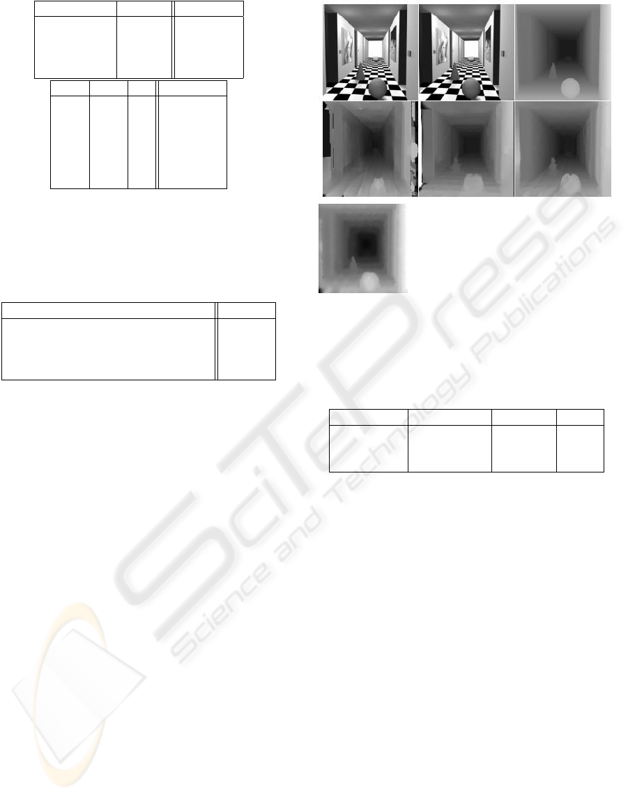
We use now the real images from the INRIA avail-

able at

Figure 7: From the left to the right and from the top to

the bottom, the stereo couple, the true disparity, the dispar-

ity from correlation algorithm, PDE from Alvarez (Alvarez

et al., 2000), method from Slesareva (N.Slesareva et al.,

2005), and ﬁnally our method. Note that the form of the

cone and the sphere are better preserved.

Noise level E Slesareva E ISLM Ratio

001 0.1952 0.1745 1.118

010 0.2529 0.2172 1.160

100 0.3297 0.26720 1.233

Figure 8: Comparison with methods from (N.Slesareva

et al., 2005) on noisy images, C =21.9215, ν =0.375,

TX = TY = V =3dt =0.3. Ratio gives E from

Slesareva divided by E from ISLM.

http://www-sop.inria.fr/robotvis/demo.

We present the three dimensions reconstruction.

ISLM convergence is more time consuming than

the other algorithms, with initial disparity found by

classical correlation algorithm it takes 6 minutes and

14 seconds to avoid 0.17 pixels precision, and 26

minutes 47 seconds to converge to 0.12 with a Pen-

tium 4). Due to our attachment term, we can not deal

with less time consuming implementation as an im-

plicit scheme. So our method seems not to be de-

signed for real time process as software but by hard-

ware and parallel implementation.

7 CONCLUSION

In this paper we have presented an iterative algorithm

for the stereo dense disparity estimation principally

based on a new attachment term. In order to give more

consistent value to the similarity measure of our itera-

LOCAL MINIMUM DISTANCE FOR THE DENSE DISPARITY ESTIMATION

347

Figure 9: Two views on Herve face, and a view on the 3D

reconstruction, ν =0.0625, C =21.75 TX = TY =7

V =3.

tive process, we use a correlation mask oriented along

the epipolar line. Then instead of taking a similarity

value as attachment term we use the distance to local

minimum obtained by the similarity. Consequently

our iterative scheme is no more linked to an energy

minimization but presents some characteristics of a

relaxation process embedding in the same framework

continuous and combinatorial aspects. The experi-

mentations show that our method convergences and

produces the best known quantitative results on im-

age benchmarks presenting continuous aspects in di-

parity values. Now we are trying our method on mid-

dlebury benchmarks. These benchmarks are different

from corridor scene because ﬁrst the disparity image

contains a lot of disparity steps, and second that the

disparities available in the middlebury benchs have

discrete values. As our algorithm gives a continuous

range of values, the error is difﬁcult to clearly inter-

pret. Links to other studies can be done, leading us to

expect again new improvements simply by the use of

other similarity measures. For example, the similar-

ity measure from (N.Slesareva et al., 2005), or (Takeo

and Okutomi, 1994) can be used in our attachment

term.

REFERENCES

Alvarez, L., Deriche, R., Sanchez, J., and Weickert, J.

(2000). Dense disparity map estimation respecting

image discontinuities: a pde and scalespace based ap-

proach.

Alvarez, L., F., G., P.L., L., and J.M., M. (1992). Ax-

ioms and fundamental equation of image process-

ing. Technical Report 9231, CEREMADE, Universit

Paris Dauphine, France, Mars 1992. Paru dans Arch.

for Rat. Mechanics 123(3), pp 199-257, 1993.

Blomgren, P. (1998). Total Variation Methods for Restora-

tion of Vector Valued Images. PhD thesis, University

of California, Los Angeles.

Boufama and Jin (2002). Towards a fast and reliable dense

matching algorithm.

Chambolle, A. (1994). Partial differential equation and

image processing. IEE Int. Conf. Image Processing,

Austin, I:16–20.

Gouet, V., Montesinos, P., and Pel

e, D. (1998). Stereo

matching of color images using differential invari-

ants. In International Conference on Image Process-

ing, Chicago, USA.

MacQueen, J. (1967). Some methods of classiﬁcation and

analysis of multivaluate observation.

Maier, D., Role, A., Hesser, J., and Manner, R. (2003).

Dense disparity maps respecting occlusions and ob-

ject separation.

Nagel, H. (1983). Constraints for the estimation of deplace-

ment vector ﬁelds from image sequences. IJCAI.

N.Slesareva, A.Bruhn, and J.Weickert (2005). Optic ﬂow

goes stereo: A variational method for estimating

discontinuity-preserving dense disparity maps.

Ohta, Y. and Kanade, T. (1985). Stereo by intra- and inter-

scanline search using dynamic programming.

Scharstein, D., Szeliski, R., and Zabih, R. (2001). A taxon-

omy and evaluation of dense two-frame stereo corre-

spondence algorithms.

Takeo, K. and Okutomi, M. (1994). A stereo matching al-

gorithm with an adaptative window : theory and ex-

periment.

Torr, P. and Murray, D. (1997). ”the development and com-

parison of robust methods for estimating the funda-

mental matrix”. International Journal of Computer

Vision, 24(3):271–300.

Zhang, Z., Deriche, R., Faugeras, O., and Luong, Q. (1994).

”a robust technique for matching two uncalibrated

images through the recovery of the unknown epipo-

lar geometry”. Technical Report RR-2273, INRIA

Sophia-Antipolis, France.

VISAPP 2006 - MOTION, TRACKING AND STEREO VISION

348