
NONPLANARITY
AND EFFICIENT MULTIPLE FEATURE EXTRACTION
Ernst D. Dickmanns, Hans-Joachim Wuensche
Institut fuer Systemdynamik und Flugmechanik, UniBw-Munich, LRT, D-85577 Neubiberg, Germany
Keywords: Image features, edge detection, corner detection, shading models.
Abstract: A stripe-based image evaluation scheme for real-time vision has been developed allowing efficient detection
of the following classes of features: 1. ‘Nonplanarity’ feature for separating image regions treatable by
planar shading models from the rest containing textured regions and corners; 2. edges and 3. smoothly
shaded regions between edges, and 4. corners for stable 2-D feature tracking. All these features are detected
by evaluating receptive fields (masks) with four mask elements shifted through stripes, both in row and
column direction. Efficiency stems from re-use of intermediate results in mask elements in neighboring
stripes and from coordinated use of these results in different feature extractors. Corner detection with
compute-intensive algorithms can be confined to a small (but highly likely) fraction of the images exploiting
the efficient nonplanarity feature. Application to road scenes is discussed.
1 INTRODUCTION
Computing power per microprocessors keeps
increasing at an almost constant rate of one order of
magnitude every 4 to 5 years. This allows combining
algorithms even for real-time vision which have
been developed for separate use some time ago. The
goal of the combined image evaluation method
presented here is: 1. to start from as few assumptions
on intensity distributions in image sequences as
possible, and 2. to re-use as many intermediate
results as possible. A rich feature set allows better
real-time understanding of dynamic scenes. Since
pixel-noise is an important factor in outdoor
environments, some kind of smoothing has to be
taken into account. This is done by fitting a planar
intensity distribution model to a local image region
if it exhibits some smoothness conditions; otherwise
the region will be characterized as non-
homogeneous. Surprisingly, it has turned out that the
planarity check for local intensity distribution itself
constitutes a nice feature for region segmentation.
Processing images in sequences of stripes allows
systematic re-use of intermediate results and
provides a nice scheme for navigation in feature
arrays for object recognition on higher system levels
(not detailed here). Most of the elementary methods
for feature extraction are not new; the reader not
acquainted with these methods can find an extensive
bibliography including text books in (Price K, USC,
Vision – Notes, bibliography, especially chapters 6
to 8). Exploiting the new “nonplanarity feature”,
they are combined in a very efficient manner. For
the same reason of efficiency, an image scaling stage
has been put upfront in which pixel intensities are
averaged over rectangular regions called ‘cells’ of
size m
c
·n
c
. These form the base for image
interpretation; image pyramid levels are subsumed
by the special case m
c
= n
c
= 2.
2 STRIPE SELECTION AND
DECOMPOSITION INTO
ELEMENTARY BLOCKS
The field size for the least-squares fit of a planar
pixel-intensity model is (2·m) by (2·n), and is called
the ‘model support region’ or mask region. For
improving re-use of intermediate computational
results, this support region is subdivided into basic
(elementary) image regions (called m
ask elements
or briefly ‘mels’) that can be defined by two
numbers: The number of cells in stripe direction m,
and normal to it (width of half-stripe) n. In figure 1,
198
D. Dickmanns E. and Wuensche H. (2006).
NONPLANARITY AND EFFICIENT MULTIPLE FEATURE EXTRACTION.
In Proceedings of the First International Conference on Computer Vision Theory and Applications, pages 198-205
DOI: 10.5220/0001370701980205
Copyright
c
SciTePress
m has been selected as 4 and n as 2; the total stripe
width thus is 4, and the total mask region is 8·4 cells.
For m = n = m
c
= n
c
= 1 the highest possible image
resolution will be obtained, however, a rather strong
influence of noise on the pixel level may show up in
the results in this case.
When working with video fields (sub-images
with only odd or even row-indices as is often done
in practical applications) it makes sense for
horizontal stripes to chose m = 2·n; this yields pixel
averaging at least in row direction for n = m
c
= n
c
= 1.
Rendering these mels as squares, finally yields the
original rectangular image shape with half the
resolution of the original full-frame. Shifting stripe
evaluation by half the stripe width only, all
intermediate mel results in one half-stripe can be re-
used directly in the next stripe by just changing sign.
The price to be paid for this convenience is that the
results obtained have to be represented at the center
point of the support region (mask) which is exactly
at cell (pixel) boundaries. However, since sub-pixel
accuracy is looked for anyway, this is of no concern.
Still open is the question of how to proceed within a
stripe. Figure 1 suggests taking steps equal to the
length of a mel; this covers all pixels in stripe
direction once and is very efficient. However,
shifting mels by just one cell in stripe direction
yields smoother (low-pass-filtered) results. For
larger mel-lengths, intermediate computational
results can be used as shown in figure 2, lower part.
The new summed value for the next mel can be
obtained by subtracting the value of the last column
(j-2) and adding the one of the next column (j+2) in
the example shown. Image evaluation progresses
top-down and from left to right.
The goal of the approach selected was to obtain
an algorithm allowing easy adaptation to limited
computing power onboard vehicles; since high
resolution is required in a relatively small part of
images only, in general in outdoor scenes, this
region can be treated with more finely tuned
parameters (foveal – peripheral differentiation).
3 REDUCTION OF A STRIPE TO
A VECTOR WITH ATTRIBUTES
The first step in mel-computation is to sum up all n
cell values in direction of the width of the half-stripe
(lower part in figure 2). This reduces the half-stripe
for search to a vector, irrespective of stripe width
specified. It is represented in figure 2 by the bottom
row (note the reduction in size at the boundaries).
All further computations are based on these values
which represent the average cell intensity at the
location in the stripe when divided by the number of
cells summed. However, these individual divisions
are superfluous computations and can be spared;
only the final results have to be scaled properly.
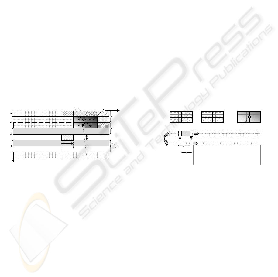
The operations to be performed for gradient
computation in horizontal and vertical direction are
shown in the upper left and center part of figure 2.
Summing two mel values (vertically in the left and
horizontally in the center sub-figure) and subtracting
the corresponding other two sums yields the
difference in (average) intensities in horizontal and
vertical direction of the support region. Dividing
these numbers by the distances between the centers
of the mels yields a measure of the (averaged)
horizontal and vertical image intensity gradient at
that location. Combining both results allows
computing absolute gradient direction and
magnitude. This corresponds to determining a local
tangent plane to the image intensity distribution for
each support region (mask) selected.
However, it may not be meaningful to enforce a
planar approximation if the intensities vary
irregularly by a large amount. For example, in the
mask of figure 3a) planar approximation does not
make sense. It shows the situation with intensities as
vectors above the center of each mel. For simplicity
the vectors have been chosen of equal magnitude on
the diagonals. The interpolating plane is indicated by
the dotted lines; its origin is located at the top of the
central vector representing the average intensity I
M
in the mask region. From the dots at the center of
each mel in this plane it can be recognized that two
+
+
- +
-
mel at position ‘j’
mel at position ‘j+1’
‘j-2’
‘j+2’
‘j ’
horizontal
gradient
vertical
gradient
resulting
mel structure
increm ental com putation of
mel-values for mels with larger
extension in stripe di rection
Step
1
f
r1
f
r2
f
c1
f
c2
+
-
+
-
-
mask center
Figure 2: Mask elements (mels) for efficient
computation of gradients and average.
1half-
stripe
stripe
‘2’
Stripe ‘1’
stripe
‘3’
1half-
stripe
center points o f
mel regions
stripe
‘4’
image region
evaluated
stripe
‘6’
half-stripe
number
1
2
3
4
5
6
.
.
m = 4
n = 2
gradient direction
me l
y,
u
z, v
Figure 1: Stripe definition (rows, horizontal) in the
operator ‘UBM2’ (cell-grid); mask elements (mels)
are defined as basic units
(
Hofmann 2004
)
.
NONPLANARITY AND EFFICIENT MULTIPLE FEATURE EXTRACTION
199
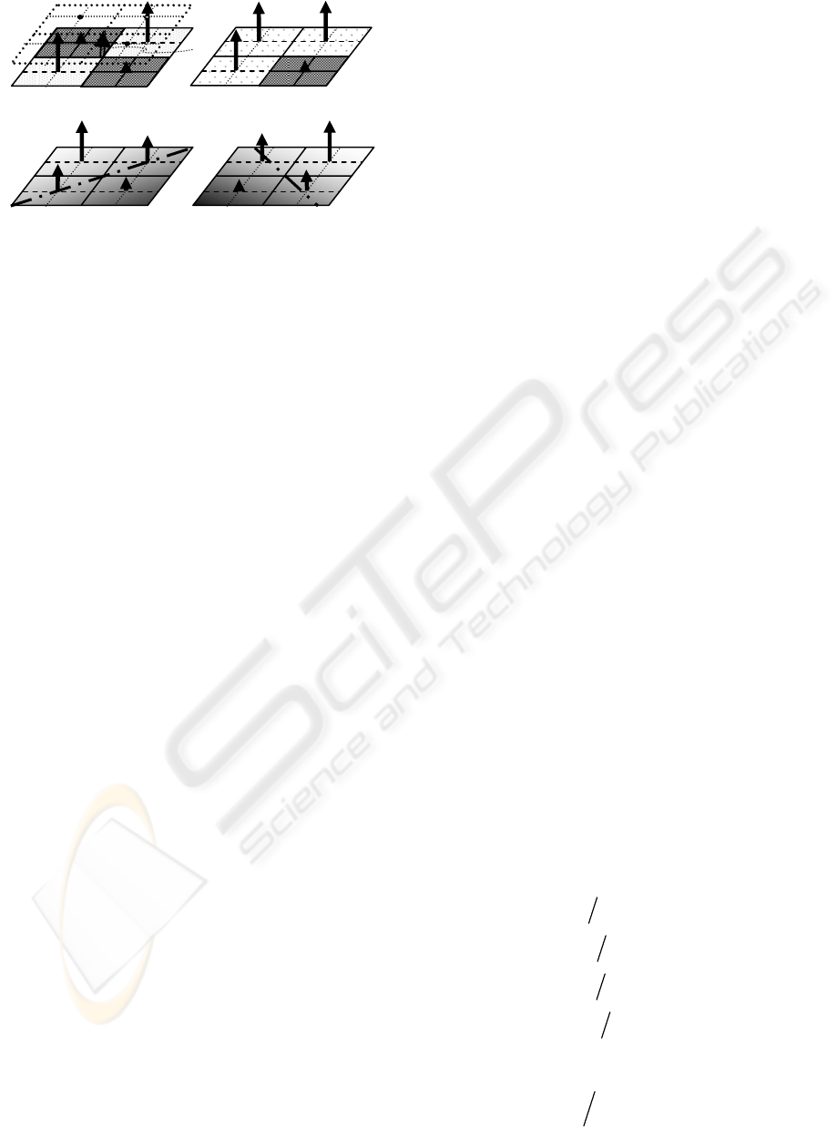
diagonally adjacent vectors of average cell intensity
are well above, respectively below the interpolating
plane. This is typical for two corners (checkerboard)
or a textured area (e.g. a saddle point).
Figure 3b) represents a perfect (gray value)
corner. Of course, the quadrant with the differing
gray value may be located anywhere in the mask. In
general, all gray values will differ from each other.
The challenge is to find algorithms allowing
reasonable separation of these feature types from
regions fit for interpolation with planar shading
models (lower part of figure 3) at low computational
costs. The goal is to segment image stripes into
regions with smooth shading, corner points, and
extended non-homogeneous regions (textured areas).
It will turn out that ‘nonplanarity’ is a new, easily
computable feature on its own (see section 5).
Corner points are of special value in tracking since
they often allow determining optical feature flow in
image sequences if robustly recognizable.
Stripe regions fit for approximation by sequences
of shading models are characterized by their average
intensities and their intensity gradients. By
interpolation of results from neighboring masks,
extreme values of gradients including their
orientation are determined to sub-pixel accuracy.
Note that, contrary to the previous standard method
KRONOS (Mysliwetz, 1990; Dickmanns Dirk, 1992
)
referred to here in the sequel as ‘UBM1’, no
direction has to be specified in advance; the
direction of the maximal gradient is a result of the
interpolation process. For this reason the method
UBM2 is called ‘direction-sensitive’ (instead of
‘direction selective’ in the case of UBM1). It is
therefore well suited for initial (strictly ‘bottom-up’)
image analysis with the ‘Hofmann-operator’
(Hofmann, 2004), while UBM1 is very efficient once
predominant edge directions in the image are known
and their changes can be estimated by the 4-D
approach (Dickmanns, Wuensche, 1999).
4 INTERPOLATION OF AN
INTENSITY PLANE IN A MASK
Average image intensities I
c,ij
within ‘cells’ of size
m
c
· n
c
are assumed to have been computed
beforehand. Cells are used to generate multiple scale
images, like e.g. (2∗2) pyramid images of reduced
size and resolution for efficient search of larger-
scale features. When working with video-fields,
cells of size 2 in row and 1 in column direction will
bring some smoothing in row direction and lead to
much shorter image evaluation times. When coarse-
scale results are sufficient, as for example with high-
resolution images for regions nearby, cells of size 4
by 2 efficiently yield scene characteristics for these
regions, while for regions further away full
resolution m
c
= n
c
= 1 can be applied in much
reduced image areas; this focal – peripheral
differentiation contributes to efficiency in image
sequence evaluation. The region of evaluation at
high-resolution may be directed by an attention
focusing process on a higher system level based on
results from a first coarse analysis (in the present or
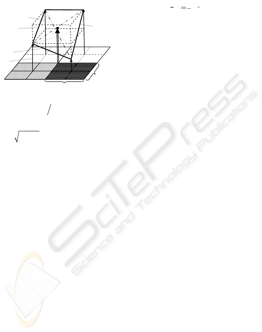
in previous images). Define I
mel,sum,ij
as sum of m · n
(average) cell intensities at location i, j in the mask
and I
M
as average of these values
,,11 ,,12
,,21 ,,22
(
)/4
M mel sum mel sum
mel sum mel sum
II I
II
=
++
+
(1)
there follows for the four normalized mel-intensities
in figure 2, top right:
,,
/.
ij mel sum ij M
I
II
=
(2)
Their sum adds up to 1. From sequences of these
four numbers of order of magnitude ‘1’ the
following features as symbolic descriptors for
transition from image data to objects perceived is
derived: : 1. ‘Planar shading’ models, 2. ‘edges’, 3.
‘textured areas’ (nonplanar elements) and 4.
‘corners’.
Figure 4 shows the local gradients in row (index
r) and column direction (index c) which play a
central role in determining these features. The
(normalized) gradients in a mask then are:
1
r
f
(
)
12 11
IIm=− (upper row) (3a)
2
r
f
(
)
22 21
IIm=− (lower row) (3b)
1
c
f
(
)
21 11
IIn=− (left column) (3c)
2
c
f
(
)
22 12
IIn=− (right column) (3d)
The global gradient components of the mask in row
and column direction then are
r
f
(
)
12
rr
ff 2=+ (global row); (4a)
I
M
a
)
b)
c)
d)
Figure 3: Feature types detectable by the method
‘UBM2’ in stripe analysis.
VISAPP 2006 - IMAGE ANALYSIS
200
c
f
(
)
12
cc
ff 2=+ (global column). (4b)
The normalized global gradient and its angular
orientation are obtained as
22
rc
gff=+
and
(
)
cr
arctan f / fα=
. (5)
Adaptation of a planar shading model in mask
area: The origin for the planar approximation
function to the discrete intensity values (~ tangent
plane) is chosen at the center of the mask area where
all four mels meet. The model of the planar intensity
approximation with the least sum of errors squared
in the four mel-centers has the yet unknown values
I
C
, g
u
and g
v
(intensity at the origin and gradients in
u- and v-direction). According to this two-
dimensional linear model, the intensities at the mel-
centers are computed as functions of the unknown
optimal parameters:
11p 0 u v
12p 0 u v
21p 0 u v
22p 0 u v
I I g m/2 g n/2
I I g m/2 g n/2
I I g m/2 g n/2
I I g m/2 g n/2
=− −
=+ −
=− +
=+ +
(6)
Let the measured values from the image be
11 12 21
I,I,I
µµµ
and
22
I
µ
. Then the errors
ij
e = I
ijp
– I
ijµ
can be written: (7)
11
11
0
12
12
u
21
21
v
22
22
I
e
1m/2n/2
I
I
e
1m/2n/2
g
e
1m/2n/2 I
g
e
1m/2n/2
I
µ
µ
µ
µ
⎡
⎤
=− −
⎡⎤
⎡⎤
⎢
⎥
⎡⎤
⎢⎥
⎢⎥
=+ −
⎢
⎥
⎢⎥
⎢⎥
⎢⎥
−
⎢
⎥
⎢⎥
⎢⎥= − +
⎢⎥
⎢
⎥
⎢⎥
⎢⎥
⎢⎥
⎣⎦
=+ +
⎢
⎥
⎣⎦
⎣⎦
⎣
⎦
In order to minimize the sum of the errors squared,
this is written in matrix form
eApI
µ
=
−
. (8)
The sum of the errors squared is
T
ee
and shall
be minimized by proper selection of
[
]
T
0uv
Igg p=
. (9)
The well known solution via pseudo-inverse is
T1T
p(AA)AI
−
µ
= , (10)
which finally yields
[][]
TT
T
0uv rc
pIgg 1ff==
. (11)
According to eqs. (1) and (2) the 1 as first
component of p means that the origin of the
interpolating plane with least squares error sum has
to be chosen as the average intensity of the mask I
M
.
5 RECOGNIZING TEXTURED
REGIONS
By substituting eq. (11) into (7), forming (e
12
– e
11
)
and (e
22
– e
21
) as well as (e
21
– e
11
) and (e
22
– e
12
),
and by summing and differencing the results, one
finally obtains
e
21
= e
12
and e
11
= e
22
; (12)
this means that the errors on each diagonal are equal.
With eqs. (1 and 7) the sum of all errors e
ij
is zero.
This means that the errors on the two diagonals have
opposite signs, but their magnitudes are equal!
These results allow an efficient combination of
feature extraction algorithms by forming the four
local gradients after eq. (3) and the two components
of the gradient within the mask after eq. (4). All four
errors of a planar shading model can thus be
determined by just one of the four Eqs. (7), that is by
2 multiplications and 4 additions/subtractions. The
planar shading model is used when the residues are
|e
ij
| < ε
pl,max
(dubbed ‘MaxErr’). (13)
From typical road scene images 96 to 99 % of all
masks yield errors |e
ij
| < 5 % and more than 99 % of
all masks yield errors |e
ij
| < 10 % (see Table 1 for
detailed results). For the rest of the cases, different
feature classes have to be applied; they cannot
reasonably be approximated by planes. The
threshold level MaxErr can be chosen from
experience in the task domain and should be selected
according to the amount of smoothing desired by the
parameters m, n, m
c
and n
c
.
It can be noticed from Table 1 that the number
of non-planarity features in column search is usually
much higher than in row search. Releasing the
threshold MaxErr from 5 % to 7.5 % reduces the
number of remaining nonplanarity features to less
Figure 4: Intensity representations in mask region
with four mask elements I
i
j
; local gradients f
kl
.
I
21
f
r2
f
c2
f
r1
= 0
f
c1
I
0
I
11
I
12
I
12
I
21
I
11
I
22
n
m
NONPLANARITY AND EFFICIENT MULTIPLE FEATURE EXTRACTION
201
than one half, in general. Note that 2½ % intensity
corresponds to about 6 gray levels out of 256 (8 bit).
Figure 5 shows results for the finest resolution
possible, where a mask element is identical to a
pixel (rows 1 and 2 in Table 1, images afterwards
2:1 horizontally compressed). Comparing this case
(1111) to the following one (3321) shows that the
absolute number of non-planarity features is higher
even though the number of mels is cut in half by the
cell size m
c
= 2, n
c
= 1. Due to the averaging process
over a larger area, apparently the local nonlinearity
in the mask area has been increased (more pixels
averaged).
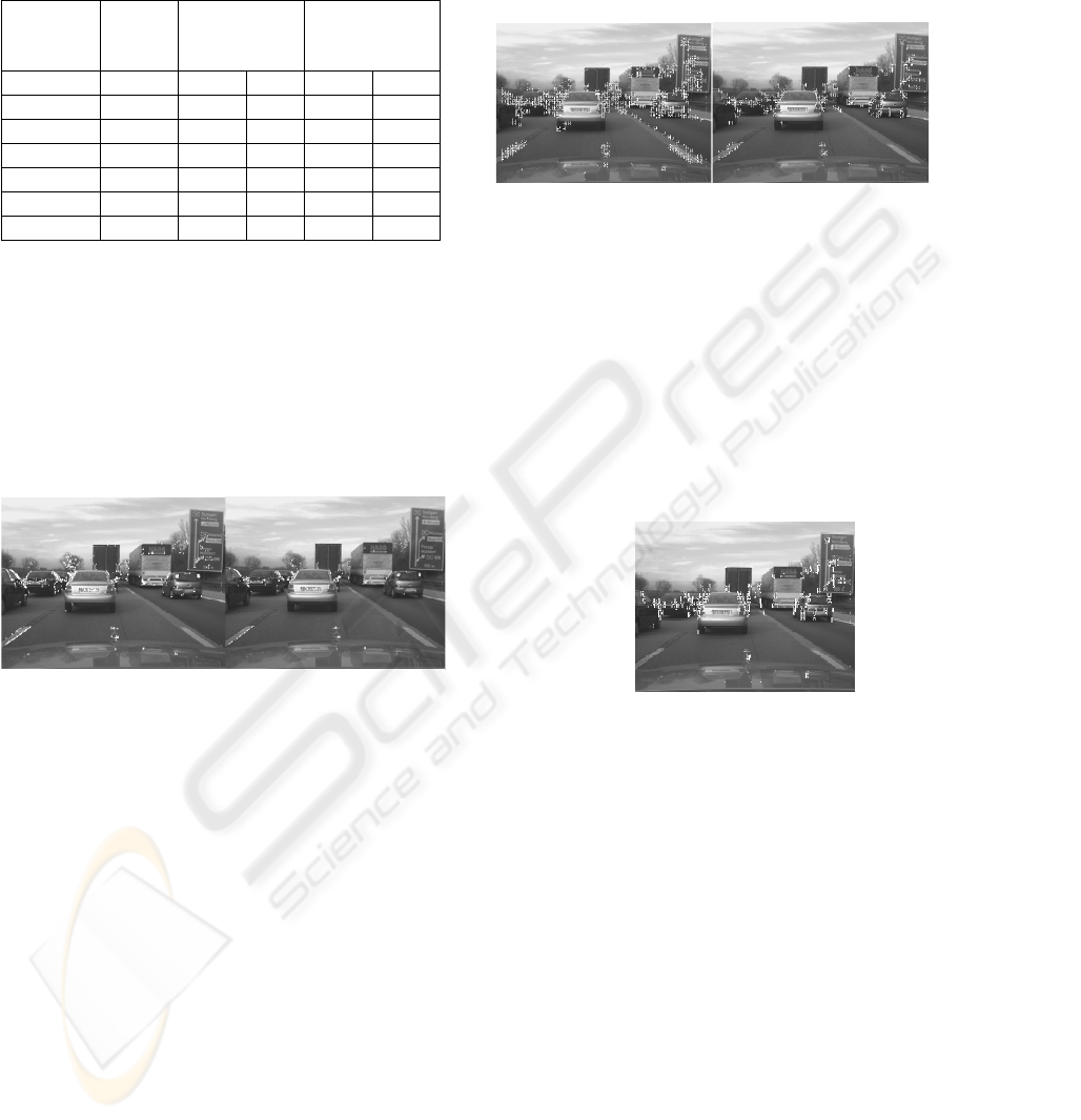
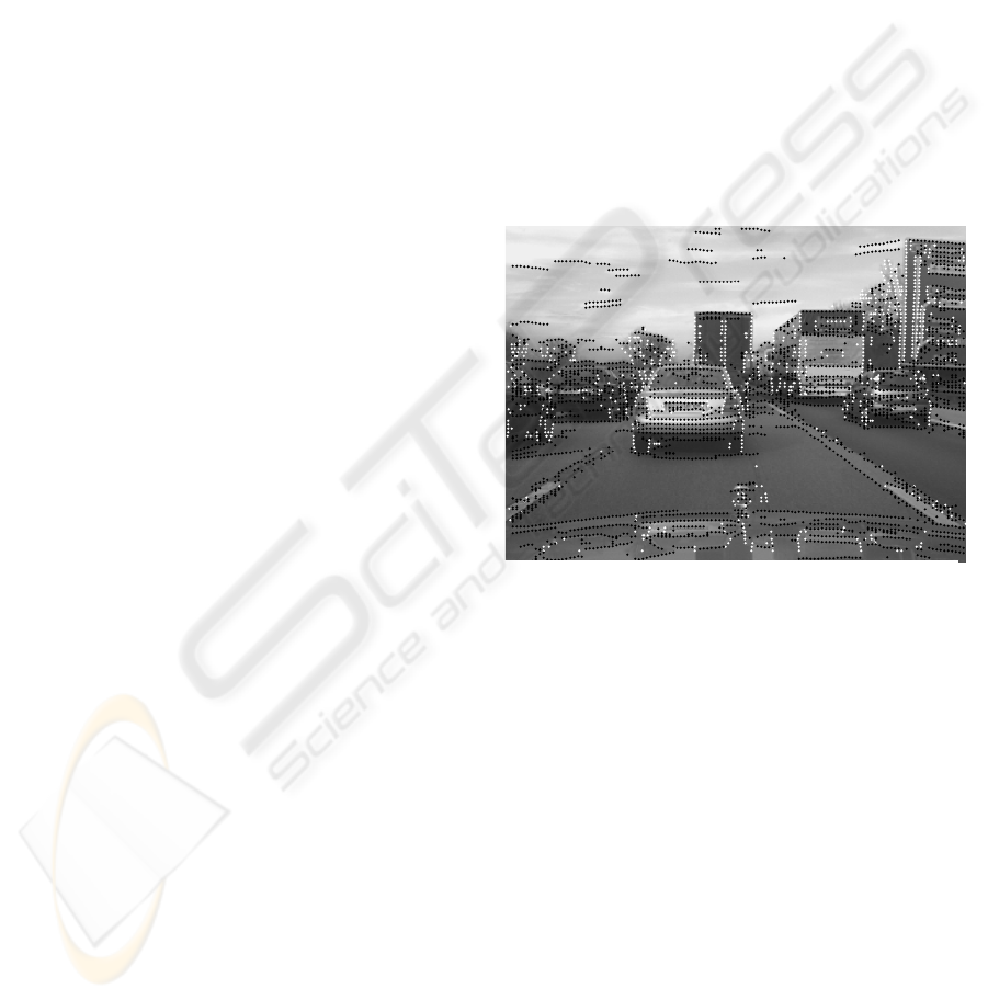
Figure 6 shows two ‘nonplanarity’ feature sets
from both row- and column- search with error
thresholds set to 5 and 7.5 % (cell size m
c
= 2, n
c
= 1,
mel size 3·3, corresponding to rows 3 and 4 in Table
1). The reduction in number of features is
immediately recognized; the locations of occurrence
remain almost the same, however. These are the
regions where stable features for tracking, avoiding
the aperture problem (sliding along edges) are more
likely to be found.
Since computing time decreases with the number
of cells as basis for forming the mask elements, this
means that nonplanarity features may be an efficient
means for tracking points of interest even in reduced
images. All significant corners for tracking are
among the nonplanarity features. They can now be
searched for with more involved methods, which
however, have to be applied to a much reduced set
of candidate image regions (a few percent only, see
table 1 and section 8).
Figure 7 shows results corresponding to row 6 of
table 1; here, the image has been reduced first to the
next higher (2·2) pyramid level, decreasing the
number of cells to one fourth the number of pixels.
F
i
g
u
r
e
7
:
‘
N
o
n
Then, the image is analyzed with stripe width 2 and
mel size of 2·2 cells, corresponding to 4·4 pixels in
one mel and 16·16 pixel in the total mask region of
the original video field. As can be seen immediately,
the regions of corner-type features for tracking
without aperture problems are the same as for the
fine resolution in figure 5; only the fine-grain
corners are gone here.
However, computing time with the large masks
is reduced by more than one order of magnitude. At
7.5 % error level the relative frequency of feature
occurrence (in percent of mels) has increased. This
m, n,
m
c
, n
c
thresh.
MaxErr
%
row search
feature | % of
number | mels
column search
feature | % of
number | mels
1 1 1 1 5 1 291 0.59 2 859 1.3
1 1 1 1 7.5 470 0.21 1 113 0.51
3 3 2 1 5 1 553 1.42 3 136 2.86
3 3 2 1 7.5 655 0.60 1 232 1.13
2 2 2 2 5 881 1.62 2 132 3.92
2 2 2 2 7.5 389 0.72 920 1.69
2 2 2 2 10 216 0.40 455 0.84
Table 1: Statistical results of ‘nonplanarity’ features
in a typical highway scene.
Figure 5 ‘Nonplanarity’ features in original video-
field as function of threshold MaxErr (cell size m
c
= 1,
n
c
= 1, mel size 1·1, finest possible resolution ~ 250 x
740 pixel). Top MaxErr = 5 %; 1291 features in row-,
2859 in column search (0.59 % resp. 1.3 % of pixels).
Bottom MaxErr = 7.5 %; 470 features in row-, 1113
in column search (0.214 % resp. 0.51 %).
Figure 6: Distribution of ‘nonplanarity’ features in a
typical highway scene. Left: threshold ErrMax = 5
%; right: ErxrMax = 7.5 %. Results from row- and
column-search are super-imposed (horizontal and
vertical white line elements); cell size m
c
= 2, n
c
= 1,
mel size 3*3.
Figure 7: Nonplanarity’ features on first pyramid
level of original video-field (cell size m
c
= 2, n
c
= 2,
yielding 125 x 370 cells). Mel size = 2*2 cells; even
with these parameters, reducing
computing time by more than an order of magnitude,
the same image regions with stable features for
tracking are found (on larger scales only). [Image
compressed 2:1 horizontally after feature
extraction.].%
VISAPP 2006 - IMAGE ANALYSIS
202
gives a hint for efficient corner search: Find regions
of interest on a larger scale first; then, for precise
localization of these features, look with higher
resolution in the regions found. The smaller corner
features missed initially are likely to be less stable
under varying aspect conditions. More experience
with this approach in different real road scenes has
to substantiate these suppositions.
6 EDGES FROM GRADIENT
COMPONENTS IN SEARCH
DIRECTION
During the planarity tests discussed above, the
gradient values of the least squares fit to the
intensity function in a mask region have been
determined (eqs. 3, 4, 11). Edges are defined by
extreme values of the gradient function in search
direction. These can easily be detected by computing
the differences of two consecutive values in search
direction and by multiplying them. If the sign of the
product is negative, an extreme value has been
passed. With parabolic interpolation from the last
three values, the location of the extreme value can
be determined to sub-cell accuracy. This indicates
that accuracy is not necessarily lost when cell sizes
are larger than single pixels; if the signals are
smooth (and they become smoother by averaging
over cells) the locations of the extreme values may
be determined to better than one tenth the cell size.
Mel-sizes of several pixel in length and width
(especially in search direction), therefore, are good
candidates for efficient and fast determination of
edge locations with this gradient method. Compared
with other methods for edge extraction as separate
algorithm it may not be the most efficient one; in
combination with the extraction of the other features
no comparable algorithm is known to the author.
In order to eliminate noise effects from data, the
absolute value of the maximum gradient found has
to be larger than a threshold value; this admits only
significant gradients as candidates for edges. The
larger the mel-size, the smaller this threshold should
be chosen. Proper threshold values for classes of
problems have to be determined by experimentation;
in the long run, the system should be capable of
doing this on its own, given corresponding payoff
functions. - Since edges oriented mainly in search
direction are prone to larger errors, these can be
excluded by limiting the ratio of the gradient
components allowed. When both gradient
components are equal in size, the edge direction is
45°. Excluding all cases where
|g
z
| < anglfacthor · |g
y
| in row search (a); (14)
|g
y
| < anglfactver · |g
z
| in column search (b),
with anglfact slightly smaller than 1, allows finding
all edges by combined row and column search.
(Close to diagonal edges should be detected in both
search directions leading to redundancy for cross
checking.) Sub-mel localization of edges is only
performed when all threshold conditions are
satisfied. The extreme value is found at that location
where the derivative of the gradient is zero.
Figure 8 shows one example of edge extraction with
this method. By choosing proper parameters for
mask size and threshold values for noise suppression
good results can be achieved. The road area is
almost free of edges; other objects are clearly
marked, and the lane markings nicely show up. Even
the mirror images of some objects on the motor hood
of the test vehicle VaMP (Mercedes 500 SEL) are
detected and marked (as well as the Mercedes star).
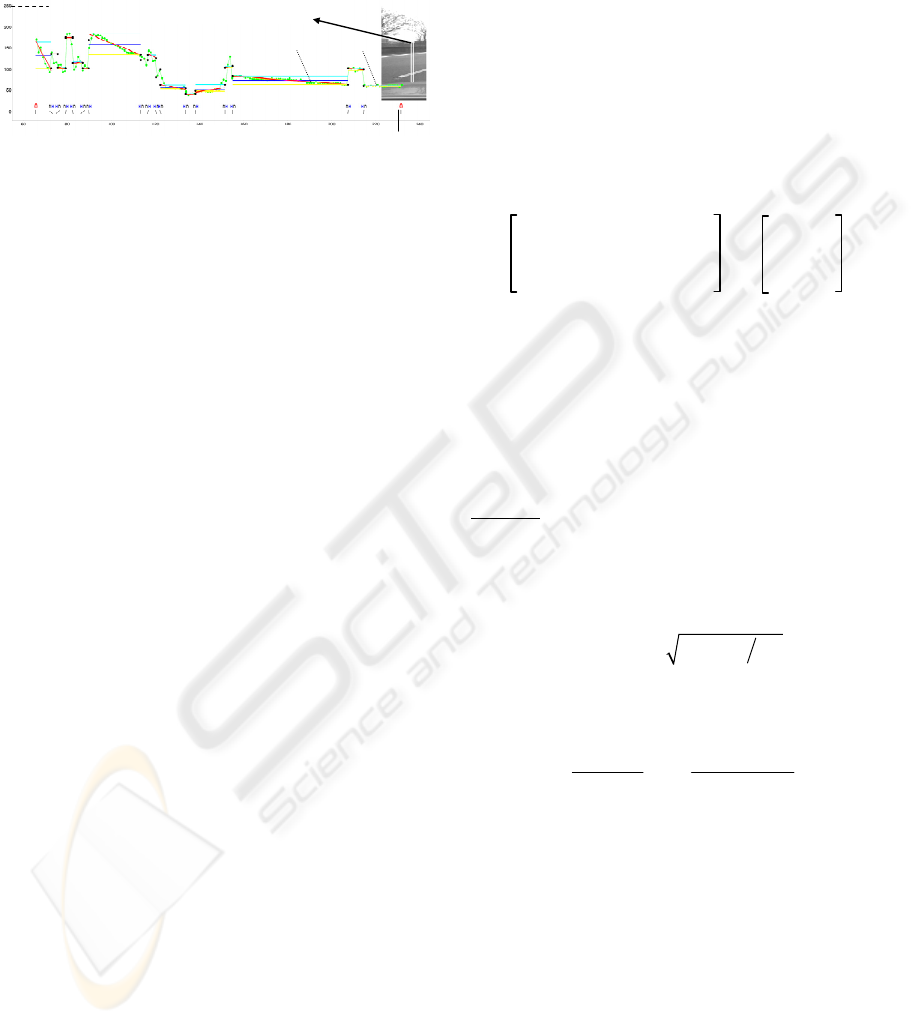
7 SHADING MODELS IN
STRIPES
Space does not allow going into any detail here; an
appreciation of what can be achieved in real time by
a single modern PC-type processor may be gained
from figure 9. The image part to the right shows part
of the original video field; neglecting sky and own
motor hood (bottom) the rectangular region marked
white is analyzed as vertical stripe. In the left part of
the figure, segmentation of the stripe is shown as
image intensity over image row number (increasing
from top to bottom like in video signals). The first
large shaded segment around row 100 is part of the
sky near the horizon; the right-hand half of the
figure represents road area with two lane markings
Figure 8: Edges from extreme values in gradient
components in row- (white) and column search
(black), [m = n = 3, m
c
= 2, n
c
= 1].
NONPLANARITY AND EFFICIENT MULTIPLE FEATURE EXTRACTION
203
as brighter regions. The MacAdam-surface of the
left lane yields the largest segment with linear
intensity shading. The centers and extensions as well
as the brightness parameters of each segment are
stored.
This is done for each vertical stripe. In this way,
intensity values of mels are transformed into lists of
segment parameters. In the following step,
neighboring areas are checked for merging edges
and homogeneous regions into larger 2-D features.
This yields extended straight edges and larger
homogeneously shaded regions. From these data
stored, the symbolically represented image can be
reconstructed as real image to show the quality of
the representation achieved (Hofmann, 2004).
The challenge in real-time vision is to find the
transition from the internal representation as
symbols in image space to objects in physical 3-D
space and time. Knowing the basic structure of
highway scenes with lanes and other objects,
hypotheses have to be generated with respect to:
where the own vehicle is on the road, where the lane
markings are (including the number and widths of
lanes actually seen), and where there are other
vehicles in the vicinity. A rich set of features
alleviates this task. The 4-D approach to dynamic
vision has been developed to solve this problem (for
a survey see [Dickmanns and Wuensche 1999];
references to detailed descriptions of the approach in
many dissertations are given there).
8 THE CORNER ALGORITHM
So-called 2-D-features designating image points
have been studied since they allow avoiding the
‘aperture problem’; it occurs for features in a plane
that are well defined in one of the two degrees of
freedom only, like edges. Since general texture
analysis requires significantly more computing
power not yet available for real-time applications in
the general case right now, we will also concentrate
on those points of interest which allow reliable
recognition, tracking and computation of feature
flow. Starting from (Moravec 1979) well known
algorithms for corner detection (among many others)
are given by (Harris CG 1988), the KLT-method by
(Birchfield S 1994; Lucas BD, Kanade T 1981;
Tomasi C, Kanade T 1991; Shi J, Tomasi C 1994)
and by (Haralick RM, Shapiro LG 1993), all based
on combinations of intensity gradients in more or
less extended regions and in several directions. The
basic ideas have been adapted and integrated into the
present algorithm dubbed ‘UBM2’.
Based on these references the following
algorithm for ‘corner detection’ fitting into the mask
scheme for planar approximation of the intensity
function has been derived and proven efficient. The
‘structural matrix’
f
r1N
² +f
r2N
² 2·f
r N
·f
cN
n
11
n
12
N = = (15)
2·f
rN
·f
cN
f
c1N
² +f
c2N
² n
12
n
22
has been defined with the terms from Eqs (3) and
(4). With the equations mentioned the determinant
of the matrix N is
2
11 22 12 11 22
11 c1 c2 22 r1 r2 r1 r2 c1 c2
det N n n n 0.75 n n
0.5 (n f f n f f ) f f f f
=
⋅−= ⋅⋅−
⋅⋅ +⋅ −
(16)
Haralick
calls det N the ‘Beaudet measure of
cornerness’, however, formed with a different term
on the cross-diagonal
12 ri ci
nff=Σ
. With the
quadratic enhancement term Q = (n
11
+ n
22
) / 2 the
two eigenvalues λ
1
and λ
2
of the structural matrix are
obtained as
2
1,2
Q1 1 detNQ
⎡
⎤
λ= ±−
⎢
⎥
⎣
⎦
. (17)
Defining λ
2N
= λ
2
/ λ
1
, Haralick’s measure of
circularity q becomes
(18)
It can thus be seen that the normalized second
eigenvalue λ
2N
and circularity q are different
expressions for the same property. In both
parameters the absolute magnitude of the
eigenvalues is lost. As threshold value for corner
points a minimal circularity q
min
is chosen as lower
limit:
. (19)
traceN = λ
1
+ λ
2
> traceN
min
may be selected as additional threshold. In a post-
processing step, within a user-defined window D,
only the local maximal value q* is selected as
corner. For larger D the corners tend to move away
min
qq>
2
2
12 2N
12 2N
4
q1 = .
(1 + )²
⎡⎤
λ−λ λ
=−
⎢⎥
λ+λ λ
⎣⎦
column 89, mel-size 1 x 3
row number in image
similarly shaded image region
image intensity
Figure 9: Result from segmentation of a single
vertical stripe in a highway scene (see image part on
ri
g
ht-hand side
)
from
(
Hofmann 2004
)
235
250
100
VISAPP 2006 - IMAGE ANALYSIS
204

from the correct position. With the definitions taken,
a double corner (like on a checker board, figure 3a)
has q = 1; a single ideal corner (figure 3b) has q =
0.75. For intensity distributions allowing good
planar approximations, q goes towards 0. The
threshold value q
min
may be adapted from experience
in the domain. Minimal circularity values for stable
corners should be set around q
min
≈ 0.7. According to
eq. (18) this yields λ
2N
values smaller than about 0.3.
When too many corner candidates are found, it is
possible to reduce their number not by lifting q
min
but by adjusting the threshold value ‘traceN
min
’
which limits the sum of the two eigenvalues.
According to the main diagonal of eq. (15) this
means prescribing a minimal value for the sum of
the squares of all local gradients in the mask. This
parameter depends on the absolute magnitude of the
gradient components and has thus to be adapted to
the actual situation at hand. It is interesting to note
that the threshold ErrMax for planarity check (eq.
13) has a similar effect as the boundary for the
threshold value traceN
min
on corners.
Figure 10 shows corners (black crosses) found
in nonplanarity regions (white bars) in vertical (left)
and horizontal search (right) on the first pyramid
level (m
c
= n
c
= 2 yielding a reduced image of about
45,000 cells). Mask size with m = n = 2 thus was 4·4
= 16 pixel. 2001 nonplanarity features (~ 4.4 % of
number of cells) with interpolation errors larger than
ErrMax = 5 % have been found in vertical search.
From these, 108 locations (dark crosses) have been
determined satisfying the corner conditions:
circularity q
min
= 0.7 and traceN
min
= 0.2 (figure 10,
left). The right-hand part of the figure shows result
of horizontal search with the same parameters except
traceN
min
= 0.15 (reduced for increasing the number
of accepted corners). 865 mask locations (~1.9 %)
yield 40 corner candidates (dark crosses). By
adjusting threshold levels, the number of corner
features obtained can be modified according to the
needs in actual applications. Combining corner
features obtained with different cell- (m
c
, n
c
) and
mel-sizes (m, n) yet has to be investigated; it is
expected that this will contribute to achieving
increased robustness.
The results in row and column search differ
mainly because stripes are shifted by half-stripe
width n (here = 2) laterally, while in search direction
masks are shifted by just one cell.
_____________________________________________________
Acknowledgement: Numerical results are based on software
derived from (Hofmann, 2004)
9 CONCLUSIONS
Checking for the goodness of planarity conditions
when fitting local linear intensity models to image
segments has led to the new ‘nonplanarity’-feature.
In typical road scenes, only 1 to 5 % of all mask
locations exceed threshold values of 3 to 10 %
planarity error (residue values). This yields an
efficient pre-selection for checking corner features.
The gradient components between the mask
elements are used in multiple ways to determine
nonplanar intensity regions, corners, edges and
segments with linear shading models. Merging of
these features over neighboring stripes leads to
larger 2-D features. Some applications to road
scenes have shown the efficiency achievable.
REFERENCES
Birchfield S 1994. KLT: An Implementation of the
Kanade-Lucas-Tomasi Feature Tracker.
http://www.ces.clemson.edu/~stb/klt/
Dickmanns Dirk 1992. KRONOS, Benutzerhandbuch,
1995, UniBwM/LRT
Dickmanns E.D.; Graefe V.: a) Dynamic monocular
machine vision. Machine Vision and Applications,
Springer International, Vol. 1, 1988, pp 223-240. b)
Applications of dynamic monocular machine vision.
(ibid), 1988, pp 241-261
Dickmanns ED, Wuensche HJ 1999. Dynamic Vision for
Perception and Control of Motion. In: B. Jaehne, H.
Haußenecker, P. Geißler (eds.) Handbook of Computer
Vision and Applications, Vol. 3, Academic Press,
1999, pp 569-620
Haralick RM, Shapiro LG 1993. Computer and Robot
Vision. Addison-Wesley, 1992 and 1993.
Harris CG, Stephens M 1988. A combined corner and
edge detector. Proc. 4
th
Alvey Vision Conference, pp.
147-153
Hofmann U 2004. Zur visuellen Umfeldwahrnehmung
autonomer Fahrzeuge. Dissertation, UniBw Munich,
LRT.
Mysliwetz B 1990. Parallelrechner-basierte Bildfolgen-
Interpretation zur autonomen Fahrzeugsteuerung.
Dissertation, UniBw Munich, LRT.
Moravec H 1979. Visual Mapping by a Robot Rover.
Proc. IJCAI 1079, pp 598-600.
Price K , (continuously). http://iris.usc.edu/Vision-
Notes/bibliography/contents.html .
Shi J, Tomasi C 1994. Good Features to Track. Proc.
IEEE-Conf. CVPR, pp. 593-600
Tomasi C, Kanade T 1991. Detection and Tracking of
Point Features. CMU-Tech.Rep. CMU-CS-91-132
NONPLANARITY AND EFFICIENT MULTIPLE FEATURE EXTRACTION
205
