LOCAL ENERGY MINIMISATIONS: AN OPTIMISATION FOR THE
TOPOLOGICAL ACTIVE VOLUMES MODEL
N. Barreira, M.G. Penedo, M. Penas
VARPA Group, LFCIA, Dpto. Computaci
´
on
Universidade da Coru
˜
na (Spain)
Keywords:
Image segmentation, 3D reconstruction, active volumes, optimisation.
Abstract:
The Topological Active Volumes (TAV) model (Barreira and Penedo, 2005) is a general active model focused
on 3D segmentation tasks. It can also be used for the surface reconstruction and the topological analysis of
the inner side of the detected objects. As any other deformable model, it defines a mesh and several energy
functions. The minimisation of the energy functions moves the mesh towards the objects in the scene. The
breaking of connections causes topological changes directed to the achievement of specific adjustments. This
way, as well as improving the adjustment, the model is able to find several objects in the image and delimit
holes in the structures detected. The TAV model achieves accurate results but the computational cost of the
segmentation procedure is high. To reduce it, this paper proposes an optimisation of the model. It consists in
performing local energy minimisations after the connection breaking process. This way, the execution times
are reduced and the accuracy of the results is increased.
1 INTRODUCTION
Active models, also called deformable models, are
widely used in image analysis to perform tasks such
as image segmentation and shape recovery. They pro-
vide a general framework that can be applied to solve
different problems in specific domains. Deformable
models were introduced in 2D as explicit deformable
contours (Kass et al., 1988) and they were generalised
to the 3D domain (Terzopoulos et al., 1988). In the re-
cent years, many deformable models have been deve-
loped to accomplish several tasks, mainly in medical
images (Ferrant et al., 2001; Zhukov et al., 2002; Liu
et al., 2003), or have been used in conjunction with
other segmentation or optimisation methods (Magee
et al., 2001; Fan et al., 2002). Nevertheless, all these
models are mainly interested in surface extraction and
shape recovery, not in the treatment of the whole de-
tected solid.
The Topological Active Volumes model (Barreira
and Penedo, 2005) is an active model focused on seg-
mentation tasks that makes use of a volumetric distri-
bution of nodes. It is fully automatic, so no a priori
knowledge is needed to initialise the model. It also
integrates information of edges and regions in the ad-
justment process and allows to obtain topological in-
formation inside the objects found. This way, the
model, not only detects surfaces as any other active
contour model, but also segments the inside of the ob-
jects. The model has a dynamic behaviour by means
of topological changes in its structure, that enables
accurate adjustments and the detection of several ob-
jects in the scene.
The main drawback of the Topological Active Vo-
lumes model is its high computational cost due to its
structure and its generality. This paper proposes an
optimisation of the model that increases its efficiency
as well as improves the results of the segmentation
process. This optimisation is based on the features of
the model and the segmentation methodology. Fur-
thermore, it can be used together with any other tech-
niques to improve the efficiency of the segmentation
procedure.
This paper is organised as follows. Section 2 des-
cribes the TAV model and the methodology used in
the segmentation process. Section 3 explains the pro-
posed optimisation method. Section 4 shows some
results of the optimisation method. Finally, the con-
clusions are exposed in section 5.
468
Barreira N., G. Penedo M. and Penas M. (2006).
LOCAL ENERGY MINIMISATIONS: AN OPTIMISATION FOR THE TOPOLOGICAL ACTIVE VOLUMES MODEL.
In Proceedings of the First International Conference on Computer Vision Theory and Applications, pages 468-473
DOI: 10.5220/0001373604680473
Copyright
c
 SciTePress

2 TOPOLOGICAL ACTIVE
VOLUMES
2.1 Model
The Topological Active Volumes (TAV) model (Ba-
rreira and Penedo, 2004) is an active contour model
focused on extraction and modelisation of volumetric
objects in a 3D scene.
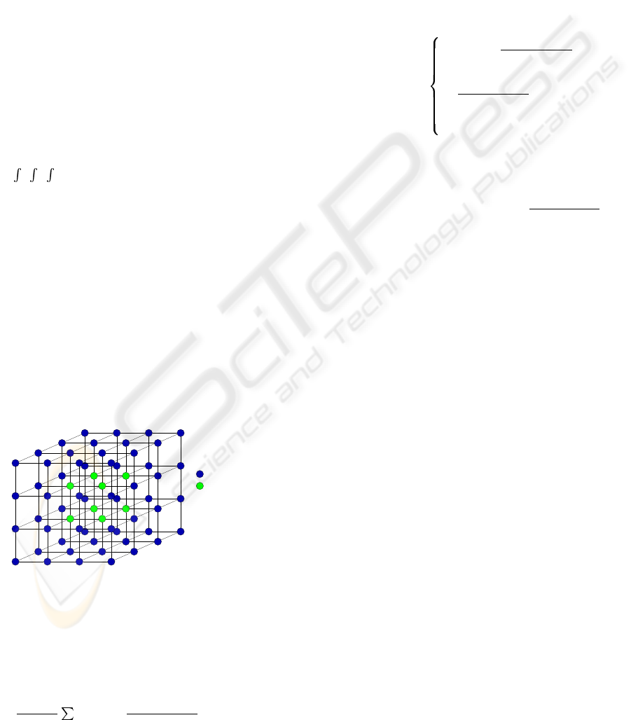
A Topological Active Volume is a three-
dimensional structure composed of interrelated
nodes where the basic repeated structure is a cube.
There are two kinds of nodes: the external nodes, that
fit the surface of the object, and the internal nodes,
that model its internal topology (figure 1). External
nodes are related to edge information and internal
nodes, to region information. The state of the model
is governed by an energy function defined as follows:
E(v(r, s, t)) =
1
0
1
0
1
0
E
int
(v(r, s, t)) + E
ext
(v(r, s, t))drdsdt
(1)
where E
int
and E
ext
are the internal and the ex-
ternal energy of the TAV, respectively. The internal
energy controls the shape and the structure of the
net. Its calculation depends on first and second or-
der derivatives that control contraction and bending,
respectively. It is defined by the following equation:
E
int
(v(r, s, t)) =
α(|v
r
(r, s, t)|
2
+ |v
s
(r, s, t)|
2
+ |v
t
(r, s, t)|
2
)+
β(|v
rr
(r, s, t)|
2
+ |v
ss
(r, s, t)|
2
+ |v
tt
(r, s, t)|
2
)+
2γ(|v
rs
(r, s, t)|
2
+ |v
rt
(r, s, t)|
2
+ |v
st
(r, s, t)|
2
)
(2)
where subscripts represents partial derivatives and α,
β and γ are coefficients controlling the first and se-
cond order smoothness of the net.
Internal nodes
External nodes
Figure 1: A TAV grid.
E
ext
represents the features of the scene that guide
the adjustment process and is different for external
and internal nodes. It is defined as:
E
ext
(v(r, s, t)) = ωf[I(v(r, s, t))]+
ρ
|ℵ(r,s,t)|
n∈ℵ(r,s,t)
1
|| v(r,s,t)−v(n)||
f[I(v(n))]
(3)
where ω and ρ are weights, I(v(r, s, t)) is the in-
tensity value of the original image in the position
v(r, s, t), ℵ(r, s, t) is the neighbourhood of the node
(r, s, t) and f is a function of the image intensity,
which is different for both types of nodes. For ex-
ample, if the objects to detect are light and the back-
ground is dark, the energy of an internal node will be
minimal when the node is on a point inside the ob-
ject with a high grey level whereas the energy of an
external node will be minimal when the node is on a
discontinuity and on a dark point outside the object.
In this situation, function f is defined as follows:
f[I(v(r, s, t))] =
For internal nodes:
h[I
max
− I(v(r, s, t))
N
]
For external nodes:
h[
I(v(r, s, t))
N
+
ξ(G
max
− G(v(r, s, t)))]
+DG(v(r, s, t))
(4)
ξ is a weighting term, I
max
and G
max
are the ma-
ximum intensity values of image I and the gradient
image G, respectively, I(v(r, s, t)) and G(v(r, s, t))
are the intensity values of the original image and gra-
dient image in the position v(r, s, t),
I
N
(v(r, s, t)) is
the mean intensity in a N × N × N cube and h is
an appropriate scaling function. DG(v(r, s, t)) is the
distance from the position v(r, s, t) to the nearest po-
sition in the gradient image that points out an edge.
2.2 Methodology
The TAV model is automatic, so the initialisation does
not need any human interaction, opposed to other de-
formable models. The mesh is placed over the whole
image and the nodes are located in such a way that
the internodal distance is the same in each dimension.
This way, the model can detect objects placed in dif-
ferent positions of the 3D image.
The adjustment process consists in the global
energy minimisation of the mesh. A greedy algorithm
is used for this task. The energy value for each TAV
node is computed in several positions of the 3D image
(the current position and its 26 neighbour positions)
at every step of the minimisation process and the best
one is chosen as the next position of the node. Once
the mesh reaches a stable situation, this is, when the
energy of each TAV node is minimal, the number of
nodes is recomputed in order to adapt the TAV size
to the object size. After that, the energy is minimised
again.
To achieve a perfect adaptation, topological
changes are performed in the mesh. These changes
consist in connection breakings between external
nodes badly placed, this is, external nodes that are not
on the surfaces of the objects. The breaking of con-
nections allows a perfect adjustment to the surfaces
LOCAL ENERGY MINIMISATIONS - An Optimisation for the Topological Active Volumes Model
469

and the detection of holes and several objects in the
3D scene. After each connection breaking, the TAV
energy is globally minimised (Barreira and Penedo,
2005).
If there were several objects in the scene, a subTAV
would be created for each one of them. A subTAV
behaves like a TAV and repeats the process described
above (Barreira and Penedo, 2004).
Figure 2 summarises the main stages of the TAV
segmentation process.
TAV
Initialization
Energy
Min.
TAV
Readjustment
Energy
Min.
Connection
Breaking
Energy
Min.
end
External
Nodes Badly
Placed?
no
yes
Figure 2: Main stages of the TAV segmentation process.
3 LOCAL ENERGY
MINIMISATIONS
The global energy minimisation is an expensive task
as it analyses every node in the mesh. On one hand, if
the node is in a wrong position with a high energy
value, it will be moved to another position with a
lower energy value. On the other hand, if the node
is correctly placed, it will stay in its current posi-
tion. In both cases, a high number of computations
will be performed but only the former computations
are useful. So, performing only useful computations
can improve the efficiency of the energy minimisation
stages.
The minimisation stages after the initialisation and
the readjustment phases (figure 2) cannot take advan-
tage of this optimisation because most of the nodes
are wrongly placed as the mesh was initiated in the
previous stage and was not adjusted to the object.
However, after each connection breaking stage there
is another energy minimisation phase and, in this
case, most of the TAV nodes are correctly placed since
the energy of the mesh has been previously minimi-
sed. This way, the optimisation will be focused on
the energy minimisation stages after the connection
breakings. These minimisations are local because
they are centred in the area where the connections are
broken.
The key issue in the local energy minimisation pro-
cedure is the selection of the node set to minimise.
The energy equations and the relationships between
nodes have been analysed in order to determine this
set.
The energy of the node depends on the own node
and its neighbours (equation 3). This implies that
once the TAV energy is minimised, the node ener-
gies will not change unless some topological change
that modifies the neighbourhood relationships among
nodes is performed in the mesh. Then, if a connection
is broken, the involved nodes will change its energy
because they lose a neighbour, so their energies have
to be minimised in order to find better positions for
them. Moreover, if a node changes its position, the
value of the function f can change because it depends
on the position of the node (equation 4). If f modi-
fies its value, not only the node will change its energy
(equation 3), but also its neighbours will be affected
since this f value is used to compute their energies
(equation 3).
(a) (b)
(c)
Node that has changed its
position when its energy
was minimisated
Connection breaking
Node in the minimisation se
t
Figure 3: Nodes in the local minimisation set. (a) After
the connection breaking. (b) After the first local energy mi-
nimisation step. The marked node has changed its position
and its neighbours are added to the minimisation set. (c) Af-
ter the second local energy minimisation step. The marked
nodes have changed their positions so their neighbourhoods
are included in the set.
As a result, the local energy minimisation proce-
dure consists of the following steps:
1. Initialise a set with the nodes involved in the con-
nection breaking
2. While the TAV energy is not minimal
(a) For each node in the set
i. Check several positions in order to minimise
the node energy
VISAPP 2006 - IMAGE ANALYSIS
470

ii. Select the best position for the node
iii. If the node has changed its position, mark its
neighbours
(b) Add the marked neighbours to the set
Figure 3 shows an example of how the local energy
minimisation method selects the nodes to perform the
energy minimisation.
4 RESULTS
The local energy minimisation procedure was tested
with several sets of 3D synthetic images and it was
compared to the global energy minimisation method.
To this end, each image was segmented by means of
several TAV meshes using both methods. The same
parameter set was used in each segmentation process
and was empirically selected. This section presents
some results obtained from both methods.
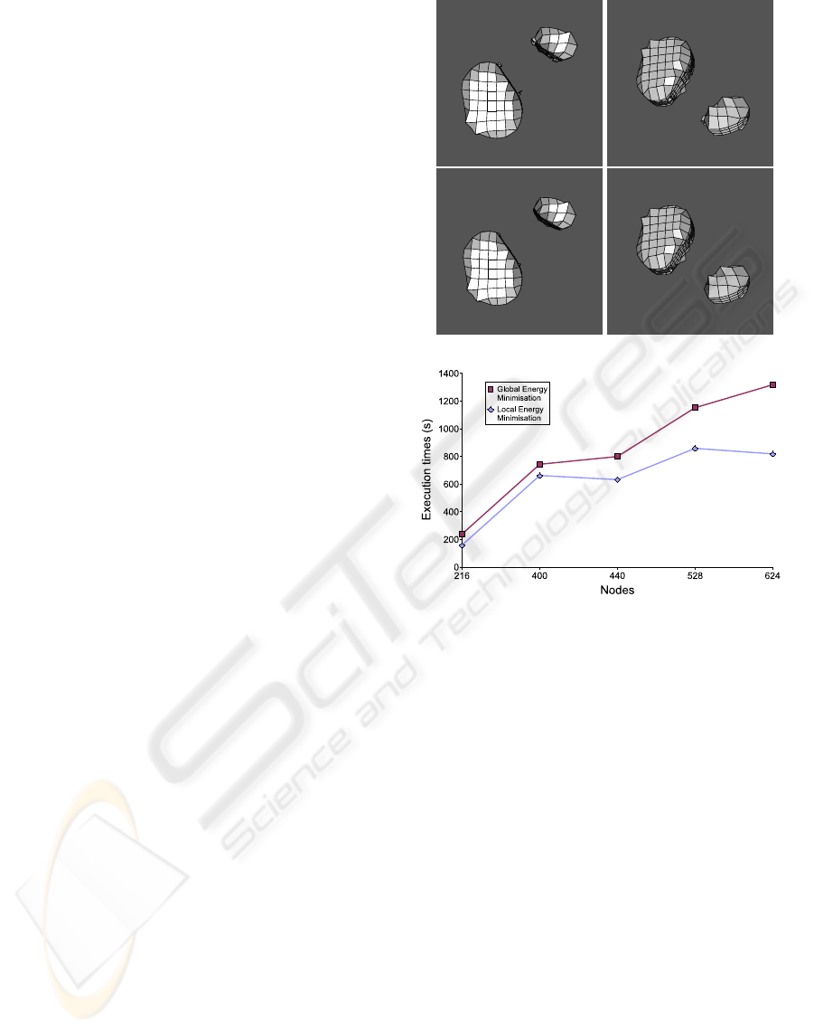
The first example is a 3D image with two objects. It
was segmented using TAVs with 216, 400, 440, 528,
and 624 nodes. The parameter set used was α =2.5,
β =0.00001, γ =0.00001, ω =3.0, ρ =4.0, and
ξ =5.0. The Sobel filter was applied to each 2D
slice to obtain the gradient image. Figure 4 shows
the results of the segmentation process and the exe-
cution times of the global and local energy minimi-
sation methods. The local method’s execution times
are always smaller. However, with small meshes, it
is common that a local minimisation affects to all the
nodes so the time differences are not significant. But,
as the number of nodes grows, the time differences
are increased.
The second example is more complex than the first
one. It was segmented with larger TAV meshes (729,
1728, 2744, 4096, and 5832 nodes). The parameter
set used was α =3.0, β =0.00001, γ =0.00001,
ω =3.0, ρ =3.0, and ξ =5.0. The gradient image
was obtained with a 3D Canny filter (Canny, 1986).
Figure 5 shows several views of the segmented fi-
gure and the execution times for the global and local
energy minimisation methods. In this example, the
execution times of the local method are lower, too.
Figure 6 shows the results of another segmentation
example. The object was segmented using TAVs with
180, 847, 2304, and 4800 nodes. The values of the pa-
rameters were α =3.5, β =0.00001, γ =0.00001,
ω =4.0, ρ =3.0, and ξ =5.0. The gradient image
was obtained with a 3D Canny filter (Canny, 1986). In
this example, the execution times of the local method
are also lower than the execution times of the global
method, as the chart in last row of figure 6 shows.
Figure 7 shows the results of another test set. The
object was segmented using TAVs with 847, 1521,
2560, and 3564 nodes. The values of the parameters
were α =3.5, β =0.00001, γ =0.00001, ω =3.0,
Figure 4: Results obtained on a simple example. The first
and second rows show the surface reconstruction of the ob-
jects. They were segmented using a TAV with 824 nodes.
The first row shows the results of the global energy mini-
misation and the second row, the results of the local energy
minimisation. Last row shows the execution times of both
methods using different TAV sizes.
ρ =3.0, and ξ =5.0. The gradient image was ob-
tained with a 2D Sobel filter. Like the previous ex-
amples, the execution times of the local method are
also lower than the results of the global method, as
the chart in last row of figure 7 shows.
In each example, the results obtained by the alter-
native methods are very similar. Nevertheless, the lo-
cal energy minimisation method obtains better results
in most cases since the global minimisation method
analyses the nodes in a sequential order whereas the
local minimisation method follows a recursive order:
first, the nodes involved in a connection breaking mi-
nimise their energies, then their neighbours, then the
neighbours of these neighbours, and so on. This fact
allows the mesh to achieve a natural adaptation to the
surfaces which improves the adjustment. The final
energy of the mesh can be used to measure the adjust-
LOCAL ENERGY MINIMISATIONS - An Optimisation for the Topological Active Volumes Model
471

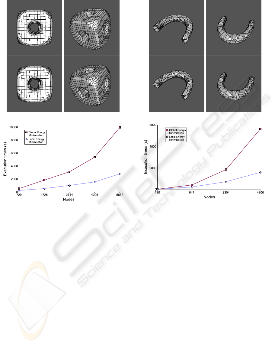
Figure 5: Results obtained on a complex example. The first
and second rows show the surface reconstruction of the ob-
ject using the global minimisation and the local minimisa-
tion, respectively. The object was segmented using a TAV
with 4096 nodes. Last row shows the execution times of
both methods using different TAV sizes.
ment of the TAV to the target object since the adjust-
ment process is an energy minimisation process. This
means that a lower energy value indicates a better ad-
justment. Table 1 shows the normalised final energies
of the meshes used for the test sets. Most of the values
obtained with the local energy minimisation method
are lower than the values obtained with the global
method, so the adjustment with the local method is
generally more accurate than the adjustment with the
global method.
5 CONCLUSIONS
This paper presents an optimisation of the TAV
model. It consists in performing local energy minimi-
sations after each connection breaking stage instead
Figure 6: Results obtained on another test set. The surface
reconstruction of the object is shown in the first and second
rows. The object was segmented using a TAV with 4096
nodes. The first row shows the results of the global energy
minimisation and the second row, the results of the local
energy minimisation. Last row shows the execution times
of both methods using different TAV sizes.
of global energy minimisations. This way, the num-
ber of useless computations is reduced and the effi-
ciency of the segmentation process is increased. Ne-
vertheless, the efficiency of the proposed method lies
mainly on the complexity of the segmented objects.
Thus, if most of the mesh nodes are wrongly placed
due to object features, the local minimisation process
can involve the whole mesh and the behaviour of the
local approach can be equal to the global one.
The local energy minimisation method was used
together with a greedy algorithm but it can be used
with any other minimisation algorithm as it only li-
mits the set of nodes to minimise and has no influence
on the minimisation algorithm. For the same reason,
the TAV parameter set is not affected by the local mi-
nimisation process.
The local minimisation method was tested with se-
VISAPP 2006 - IMAGE ANALYSIS
472

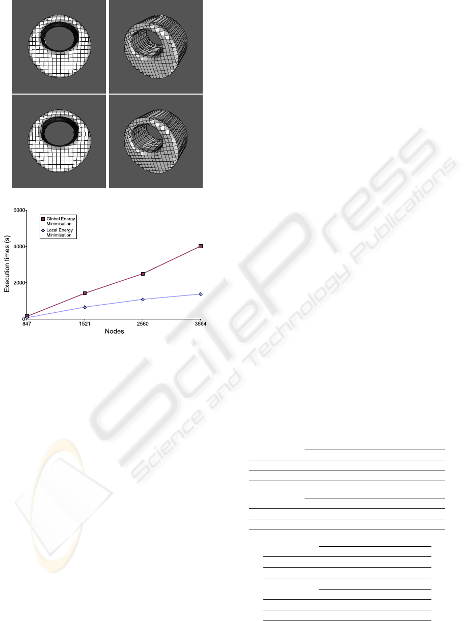
Figure 7: Results obtained on another example. The first
and second rows show the surface reconstruction of the ob-
ject. It was segmented using a TAV with 3564 nodes. The
first row shows the results of the global energy minimisation
and the second one, the results of the local energy minimi-
sation. Last row shows the execution times of both methods
using different TAV sizes.
veral sets of 3D images. The execution times were
clearly reduced and the results obtained were slightly
improved. The time differences grow exponentially
with the number of nodes since the breakings tend to
affect a lower percentage of nodes as the number of
nodes is increased.
Future work in the TAV optimisation field includes
the definition of more efficient minimisation algo-
rithms, the use of information from the domain to
guide the adjustment process when the model is ap-
plied to a specific field, and the parallelisation of the
energy minimisation stage.
REFERENCES
Barreira, N. and Penedo, M. G. (2004). Topological Active
Volumes for Segmentation and Shape Reconstruction
of Medical Images. Image Analysis and Recognition:
Lecture Notes in Computer Science, 3212:43–50.
Barreira, N. and Penedo, M. G. (2005). Topological Ac-
tive Volumes. EURASIP Journal on Applied Signal
Processing, 13(1):1937–1947.
Canny, J. (1986). A computational approach to edge-
detection. IEEE Trans. on Pattern Analysis and Ma-
chine Intelligence, 8(6):679–698.
Fan, Y., Jiang, T., and Evans, D. J. (2002). Volumetric
Segmentation of Brain Images Using Parallel Genetic
Algorithms. IEEE Transactions on Medical Imaging,
21(8):904–909.
Ferrant, M., Cuisenaire, O., Macq, B., Thiran, J., Shen-
ton, M., Kikinis, R., and Warfield, S. (2001). Surface
based atlas matching of the brain using deformable
surfaces and volumetric finite elements. In MICCAI
2001, pages pp. 1352–1353.
Kass, M., Witkin, A., and Terzopoulos, D. (1988). Active
contour models. International Journal of Computer
Vision, 1(2):321–323.
Liu, R., Shang, Y., Sachse, F. B., and Dssel, O. (2003).
3D active surface method for segmentation of medical
image data: Assessment of different image forces. In
Biomedizinische Technik, volume 48-1, pages 28–29.
Magee, D. R., Bulpitt, A. J., and Berry, E. (2001). Combin-
ing 3d deformable models and level set methods for
the segmentation of abdominal aortic aneurysms. In
BMVC.
Terzopoulos, D., Witkin, A., and Kass, M. (1988). Con-
straints on deformable models: Recovering 3D shape
and nonrigid motion. Artificial Intelligence, 36(1):91–
123.
Zhukov, L., J. Bao, I. G., Wood, J., and Breen, D. (2002).
Dynamic deformable models for mri heart segmenta-
tion. In SPIE Medical Imaging 2002.
Table 1: Normalised TAV energies obtained in the segmen-
tation processes of the examples.
TAV nodes - first example
216 400 440 528 624
Global min. 0,583 0,757 0,787 0,885 1
Local min. 0,540 0,745 0,780 0,881 0,952
TAV nodes - second example
729 1728 2744 4096 5832
Global min. 0,366 0,512 0,663 0,817 0,992
Local min. 0,365 0,511 0,665 0,816 1
TAV nodes - third example
180 847 2304 4800
Global min. 0,130 0,336 0,600 1
Local min. 0,140 0,344 0,581 0,959
TAV nodes - fourth example
847 1521 2560 3564
Global min. 0,511 0,622 0,832 1
Local min. 0,511 0,621 0,837 0,995
LOCAL ENERGY MINIMISATIONS - An Optimisation for the Topological Active Volumes Model
473