
SIMPLIFIED REPRESENTATION OF LARGE RANGE DATASET
Hongchuan Yu and Mohammed Bennamoun
School of Ccomputer Science & Software Engineering
University of Western Australia,WA 6009,Australia
Keywords: Range Dataset, Simplification, SVDecomposition, Radial Basis Functions.
Abstract: In this paper, we consider two approaches of simplifying medium- and large-sized range datasets to a
compact data point set, based on the Radial Basis Functions (RBF) approximation. The first algorithm uses
a Pseudo-Inverse Approach for the case of given basis functions, and the second one uses an SVD-Based
Approach for the case of unknown basis functions. The novelty of this paper consists in a novel partition-
based SVD algorithm for a symmetric square matrix, which can effectively reduce the dimension of a
matrix in a given partition case. Furthermore, this algorithm is combined with a standard clustering
algorithm to form our SVD-Based Approach, which can then seek an appropriate partition automatically for
dataset simplification. Experimental results indicate that the presented Pseudo-Inverse Approach requires a
uniform sampled control point set, and can obtain an optimal least square solution in the given control point
set case. While in the unknown control point case, the presented SVD-Based Approach can seek an
appropriate control point set automatically, and the resulting surface preserves more of the essential details
and is prone to less distortions.
1 INTRODUCTION
A range dataset is a picture in which each pixel
value encodes not the intensity of a usual 2D image
but rather the depth (or range) information. This type
of imagery therefore provides direct, explicit
geometric information which is useful in many
applications. However, this range dataset is usually
large-sized, non-uniformly sampled (i.e. the surface
is typically irregularly sampled, and exhibits varying
sampling densities), and contains noise or unwanted
details. The challenging problems include the
interpolation of the scattered surface dataset, the
removal of the inherent noise from the range dataset
and the simplification of this dataset for the large-
sized case. At present, the Radial Basis Functions
(RBF) are popular for interpolating scattered data
since they can effectively interpolate across large,
irregular holes in incomplete surface data without
constraining the topology of an object or any priori
knowledge of the shape (Carr et al. 2003, 2001,
1997, Morse et al. 2001). (Carr et al. 2003), further
employed RBF technique to smooth the scattered
range data. As an alternative approach, (Fleishman
et al. 2005), recently employed the Moving Least-
Squares (MLS) technique to handle noisy range
datasets. However, since these range dataset usually
contains a large data point set, this will bring about a
higher computational complexity. For example,
computing a RBF interpolation is performed by
solving an associated linear system of basis
functions of size up to (N+K)×(N+K), where N is the
number of control points and K is the number of a
low polynomial coefficients. As this system
becomes larger, the amount of computation required
to solve it grows as
)(
3
NO . In order to decrease the
computational complexity, (Beatson et al. 1999,
2001, 2000) and (Suter 1994) proposed their
individual fast evaluation approaches that have a
complexity of O(NlogN).
However, the range dataset usually contains
redundant information to represent a surface.
Considering all the points as control points to fit the
surface must lead to a higher complexity, and this is
indeed unnecessary. But how to simplify the range
dataset is still an open problem. This paper deals
with the problem of range dataset simplification, and
aims at the simplification of the RBF approximation.
To the best of our knowledge, this problem has only
been addressed by (Carr, et al. 2001), who proposed
a greedy algorithm for reducing the data point set.
Their basis idea is to use the fitting accuracy as the
criterion to choose the control points. In our works,
we prefer to pay attention to the space distribution of
the point set, since its inherent geometric properties
indicate which points are critical to represent a
172
Yu H. and Bennamoun M. (2006).
SIMPLIFIED REPRESENTATION OF LARGE RANGE DATASET.
In Proceedings of the First International Conference on Computer Vision Theory and Applications, pages 172-179
DOI: 10.5220/0001374201720179
Copyright
c
SciTePress

surface. The main contribution of this paper is to
present a novel partition-based SVD approach,
which can be employed to reduce the dimension of a
large-sized symmetric square matrix. Furthermore,
we employed this novel tool to the range dataset
simplification, and the resulting surface preserves
more essential structures and less distortion.
The remainder of this paper is organized as
follows. In Section 2, the RBF approach is first
introduced briefly. Then, we introduce two approach
of simplifying the RBF approximation in Section 3,
one is the Pseudo-Inverse Approach and other is the
SVD-Based Approach. Experiments and analysis are
shown in Section 4. Finally, Section 5 gives our
conclusions and future works.
2 RADIAL BASIS FUNCTIONS
An implicit surface is defined by an implicit
function, which is a continuous scalar-valued
function over the domain, i.e.
RRf
n
→: . Therein,
the function values of points at the implicit surface
take on zero, while the function value takes on
positive value interior to the implicit surface and is
negative outside the surface (or conversely). The
magnitude is defined as the distance from a point to
the implicit surface. This implicit function is also
called a signed distance function. Our goal is to
recover the implicit function f from a set of dataset
(or control point set). Indeed, this is an ill-posed
problem, since it has an infinite number of solutions.
The standard procedure is to obtain a solution of this
ill-posed problem from a variational principle, that
is, to minimize the following functional,
()
∑
=
+
′
−
N
i
ii
f
fff
1
2
][)(min
αφ
x , (1)
where,
n
i
R∈x is control point coordinate vector,
i
f
′
is the function value of
i
x ,
φ
[f] is a smoothness
functional (in general, the thin-plate energy
functional (Carr et al. 2001) is adopted), and α is the
regularization parameter.
An effective expression of the solution of Eq.(1) is
in terms of radial basis functions centered at the
control points. Radial basis functions are radially
symmetric about the control points, which is written
as follows,
∑∑
==
+−=
K
k
kk
N
i
ii
dGcf
11
)()()( xxxx
ϕ
, (2)
where,
)(
i
xxG − is a basis function
RRRG
nn
→×: ,
K
kk
}{
ϕ
is a basis in the K-
dimensional null space. In order to determine the
coefficients
i
c and
i
d , one can solve the following
linear system.
⎟
⎟
⎠
⎞
⎜
⎜
⎝
⎛
′
=
⎟
⎟
⎠
⎞
⎜
⎜
⎝
⎛
⎟
⎟
⎠
⎞
⎜
⎜
⎝
⎛
00
f
d
c
T
G
ϕ
ϕ
, (3)
where,
T
N
ff ),...,(
1
′′
=
′
f
, )(
jiij
GG xx
−
= ,
T
N
cc ),...,(
1
=c ,
T
K
dd ),...,(
1
=d . The basis function
is of the form
)||(||)(
2
⋅
=
⋅
GG , which includes
biharmonic spline, triharmonic spline and
multiquadric (refer to (Carr et al. 2001) for details).
The
∑
K
k
kk
d )(x
ϕ
in Eq.(2) is usually a degree one
polynomial since the thin-plate energy consist of
second order derivatives.
In the scattered data interpolation case, it is
straightforward to employ all the data points to
construct the coefficient matrix of Eq.(3) and
directly solve the coefficient vectors c and d. Herein,
all the data points are regarded as control points. For
the small-sized range datasets, this direct approach is
very useful for the direct solution of the
interpolation problem. But in the moderate- and
large-sized cases, the coefficient matrix of Eq.(3)
would exceed the computational capability of the
usual machine. Thus, the control point set has to be a
subset of the whole range dataset. Indeed, the range
dataset is usually redundant with respect to the
representation of a surface. It is unnecessary to
regard all the data points as control points.
3 SIMPLIFICATION OF RANGE
DATA
Consider the medium- and large-sized range datasets
case. In this section, we devise two approaches in
order for the solution of the implicit function f to
account for the control point set and non-control
point set.
3.1 Pseudo-Inverse Approach
In this case, the control point set is known in
advance. This means that the basis functions have
been determined and the basis of the functional
space of the implicit function f are fixed. Herein, we
only need to select an appropriate set of coefficients
i
c and
i
d for Eq.(2). This can be achieved through
minimizing the following functional,
SIMPLIFIED REPRESENTATION OF LARGE RANGE DATASET
173

⎟
⎟
⎠
⎞
⎜
⎜
⎝
⎛
′
−+
′
−
∑∑
M
j
jj
N
i
ii
f
ffff
2
2
),,(
),,(),,(min dcxdcx
dcx
, (4)
where, N is number of control points, M is number
of non-control points.
Considering Eq.(2), Eq.(3) and Eq.(4) together, one
can convert the above minimization problem as
follows,
⎟
⎟
⎟
⎠
⎞
⎜
⎜
⎜
⎝
⎛
′
′
=
⎟
⎟
⎠
⎞
⎜
⎜
⎝
⎛
⎟
⎟
⎟
⎠
⎞
⎜
⎜
⎜
⎝
⎛
M
N
MM
T
N
NN
G
G
f
f
d
c
00
ϕ
ϕ
ϕ
(5)
where,
N
f
′
and
M
f
′
are respectively the vectors of
function values of control points
i
x and non-control
points
j
x ,
N
G and
N
ϕ
are constructed by the
control points, which are described in the same
manner as in Eq.(3),
M
G and
M
ϕ
are constructed by
the non-control points, which can simply be
determined using Eq.(2) with the same control
points that are used for
N
G .
N
G is a symmetric
matrix of size N×N while
M
G is a asymmetric
matrix of size M×M. Through the pseudo-inverse of
the coefficient matrix in Eq.(5), we can obtain a
solution of
c and d in a least square sense.
The advantages of this approach are several. First,
the algorithm is easily implemented since only the
linear system of Eq.(5) needs to be solved. Second,
the error converges since we can get a least square
solution from Eq.(5). However, its deficiencies are
also obvious. From a theoretical viewpoint, the
control point set is redundant. As we knew, the basis
functions
)(
i
G xx − were non-compactly supported.
This means that the control point set is redundant
with respect to the representation of a surface.
Furthermore, because the control points are fixed,
the resulting implicit function of Eq.(2) is bounded
in the functional space spanned by the basis function
)(
i
G xx − . It is impossible to deform the implicit
function f to go beyond this original functional
space. This means that the control points should be
uniform samples over the whole domain but not the
local samples. Therefore, it is necessary to
investigate the choice of the control points. From the
perspective of an application, in large-sized range
data case, due to a large number of data points, the
coefficient matrix of Eq.(5) would quickly exceed
the computational capability of the usual machine.
In the following section, we will try to devise a
novel approach to overcome these two problems.
3.2 SVD-Based Approach
In this case, the control point set is unknown. Our
basic idea is to apply the Singular Value
Decomposition (SVD) to the coordinate set of range
data points to simplify the data points so as to obtain
some principal control points. Obviously, the first
problem we encountered will be the conflict between
the large-sized point coordinate set and the usual
limited computational capability. It is
straightforward to partition the large-sized set into a
series of subsets, and then deal with them
individually. In the following, we first explain our
novel partition-based SVD approach, then apply it to
the large-sized data point set for point simplification.
In the RBF approximation, the coefficient matrix of
Eq.(3) is real symmetric and positive semi-definite.
Our goal is to exploit these properties in order to
reduce the dimension of this square matrix. Without
loss of generality, we first give the following two
basic propositions (see (Yu et al. 2005) for a formal
proof).
Proposition 1
Let a real symmetric matrix
nn
R
×
∈A be SVD
decomposed as
T
VUA Λ= , where
0...),,...,(
11
≥≥≥
=
Λ
nn
diag
λ
λ
λ
λ
. If r≤rank(A)
and let
T
VUA
′
Λ
′′
=
′
, where
rrrn
RR
××
∈Λ
′
∈
′′
,,VU
, then,
1
2
+
=
′
−
r
λ
AA .
Proposition 2
Partitioning columns of A into r block submatrices
),...,(
1 r
AAA
=
, where riR
i
pn
i
,...,1, =∈
×
A ,
∑
=
=
r
i
i
pn
1
, we have, )()(
i
T
ii
rankrank AAA = .
Proposition 1 implies that
A
′
is an optimal
approximation of A among all rank r matrices in a 2-
norm sense. Furthermore, if rank(A)=r and r<n, this
implies that A can be partitioned into r block
submatrices and each block submatrix is expected to
be of rank 1.
Due to the real symmetry property of A, each block
partitioned along column (or row) must correspond
to a block partitioned along row (or column). For
convenience, each strip block can be compressed to
a real symmetric matrix. Proposition 2 implies that
this compressed symmetric matrix
i
T
i
AA has the
same rank as
i
A . Therefore, we are able to expect
VISAPP 2006 - IMAGE UNDERSTANDING
174

the square matrix
i
T
i
AA to be of rank 1. This
procedure is illustrated in Fig.1.
⎟
⎟
⎟
⎟
⎟
⎟
⎟
⎠
⎞
⎜
⎜
⎜
⎜
⎜
⎜
⎜
⎝
⎛
=→
⎟
⎟
⎟
⎟
⎟
⎟
⎠
⎞
⎜
⎜
⎜
⎜
⎜
⎜
⎝
⎛
=
r
T
r
i
T
i
T
T
r
T
i
T
ri
AA
AA
AA
BA
A
A
A
AAA
0
0
*...*...*
***
*...*...*
111
1
Figure 1:Real symmetric matrix A is converted to a quasi-
diagonal form B.
It can be noted that the compressed matrices
i
T
i
AA
construct a block diagonal matrix B. In other words,
the partition of A is transformed to a block diagonal
matrix B. This transform effectively simplifies the
computation burden, since the future numerical
analysis of A can be fulfilled through the individual
analysis of each symmetric block
i
T
ii
AAB = .
Applying SVD decomposition to
i
B , one can get
T
iiii
T
ii
VVAAB
2
Λ== , where the SVD of
i
A is
T
iiii
VUA Λ=
. When we let
1)()( ==
i
T
ii
rankrank AAB , the approximation of
i
B can therefore be written as,
T
iii
i
)(
1
)(
1
2
)(
1
vvB
λ
=
′
,
where
2
)(
1
i
λ
is the maximum singular value of
2
i
Λ ,
)(
1
i
v
is the column singular vector of
i
V
corresponding to
2
)(
1
i
λ
. Consequently, B can be
reconstructed by the approximations
r
BB
′
′
,...,
1
as
follows,
(
)
⎟
⎟
⎟
⎟
⎠
⎞
⎜
⎜
⎜
⎜
⎝
⎛
⎟
⎟
⎟
⎟
⎠
⎞
⎜
⎜
⎜
⎜
⎝
⎛
=
⎟
⎟
⎟
⎠
⎞
⎜
⎜
⎜
⎝
⎛
′
′
=
′
T
r
T
r
r
r
diag
)(
1
)1(
1
2
)(
1
2
)1(
1
)(
1
)1(
1
1
0
0
,...,
0
0
0
0
v
v
v
v
B
B
B
λλ
(6)
For each block
i
B , we know that
i
B is indeed the
Gram matrix of
i
A , which is symmetric and
positive definite. The diagonal difference between
i
B and its approximation
i
B
′
indicates which
column (or row) vectors of
i
A are principal basis
vectors of
i
A . This is due to the fact that each
diagonal entry of
i
B is the inner product of each
column (or row) vector of
i
A . If the ith column (or
row) vector is a principal vector of
i
A , its inner
product can be approximated by the ith diagonal
entry of the approximation
i
B
′
. One can
conveniently preserve a column (or row) of
i
A by
evaluating
ii
i
jji
i
jj
i
jj
i
jj
pjbbbb ,...,1,,,
)(
,
)(
,
2
)(
,
)(
,
=
′
∈
′
∈
′
− BB so that
these selected columns (or rows) construct an r-
dimensional matrix
rr×
A
~
, which is a dimension
reduced version of A.
Up to now, we established a partition-based SVD
approach for the large-sized real symmetric matrix
case. It can be summarized as follows.
Partition-Based SVD Approach:
1)
Convert the partitioned
()
r
AAA ,...,
1
= to
a block diagonal matrix B;
2)
Compute the approximation
i
B
′
of each
symmetric subblock
i
B in B through SVD,
in which
(
)
1=
′
i
rank B ;
3)
Compute the diagonal difference between
i
B and
i
B
′
;
4)
Select the principal vector of
i
A by
evaluating
i
i
jji
i
jj
i
jj
i
jj
bbbb BB
′
∈
′
∈
′
−
)(
,
)(
,
2
)(
,
)(
,
,, to
construct the reduced matrix
A
~
of size r×r.
However, it can be noted that the approximation
error of B can be evaluated through 2-norm of
2
BB
′
−
. Moreover, the upper bound of error can be
estimated as
2
)(
2
2
max
i
i
λ
≤
′
− BB (for details, refer
to [10]). Indeed, a good partition approach can be
deduced by minimizing the error of
2
)(
2
max
i
i
λ
. It can
also be noted that
2
)(
2
max
i
i
λ
is a variable for various
partition approaches. It can be further proven that for
the singular values of each column of A,
n
σ
σ
,...,
1
and
0...
1
≥≥≥
n
σ
σ
, there exists a partition (i.e. the
dimension of A is reduced to r) such that,
2)...(max
22
1
2
2
)(
2 nrr
i
i
σσσλ
+++≤
+
(for details, refer
to (Yu et al. 2005)). This implies that
),...,,(
1 nrr
σ
σ
σ
+
correspond to the non-principal
columns (or rows) of A respectively, and in order to
further reduce the error of
2
)(
2
max
i
i
λ
, we have to
seek a column (or row) combination of A (i.e. all the
non-principal columns or rows are left in
r
A ) so as
to obtain the minimum of
()
22
1
2
...
nrr
σσσ
+++
+
. Of
course, if the non-principal columns or rows are
distributed in each partition
i
A , this minimization
problem will be described as follows,
SIMPLIFIED REPRESENTATION OF LARGE RANGE DATASET
175
(
)
2
)(
2
)(
1
...max min
i
p
i
i
i
σσ
++ .
However, seeking the optimal partition of A is
indeed an NP-complete problem. We will present
below our partition scheme in the case of range data
simplification.
Consider a coordinate set of range data points. One
can note that the distribution of the point cloud
formed by data points is not uniform. The geometric
distribution of data points is redundant with respect
to the topological structure of a point cloud. In order
to obtain a compact data point set, we can directly
apply the SVD technique to the basis functions of
Eq.(3). Indeed, the sub-matrix G in Eq.(3) consists
of the basis functions
)(
ji
G xx − , which is a real
symmetric and positive semi-definite matrix. If there
existed a partition for G, applying the above
presented partition-based SVD approach to G, one
could easily simplify G to get a dimension reduced
version of G. But, how to partition G is still an open
problem that is covered in this section.
Considering G, one can note that the basis function
)(
ji
G xx − is a function of the Euclidean distance
ji
xx − , and )()(
ijji
GG xxxx −
=
− . The ith row
(or column) of G is a vector of
()
)(),...,(
1 iNi
GG xxxx −− about the ith point
i
x .
Herein, the geometric meaning of the singular values
of the columns (or rows) of G is that the singular
value
i
σ
of column (or row) i of G is a
measurement of the divergence of the data point set
to the ith data point
i
x , i.e. the bigger the singular
value
i
σ
is, the farther the data point set departs
from the ith data point
i
x . In terms of proposition 2,
the r columns (or rows) of G with the first r
maximum singular values of columns should be put
into r different partitions of G. It is clear that the
resulting partition of G through the selection of
points with the larger divergence as the centers of
the different partitions can minimize the residual
error between G and its approximation
G
′
.
However in our case, G is not approximated by the
same dimension of
G
′
but its dimension is reduced
(i.e. the number of control points needs to be
reduced). Obviously, the reduction of the control
points will lead to the loss of some details. If only
the points with the largest divergence are
considered, many details will have to be abandoned.
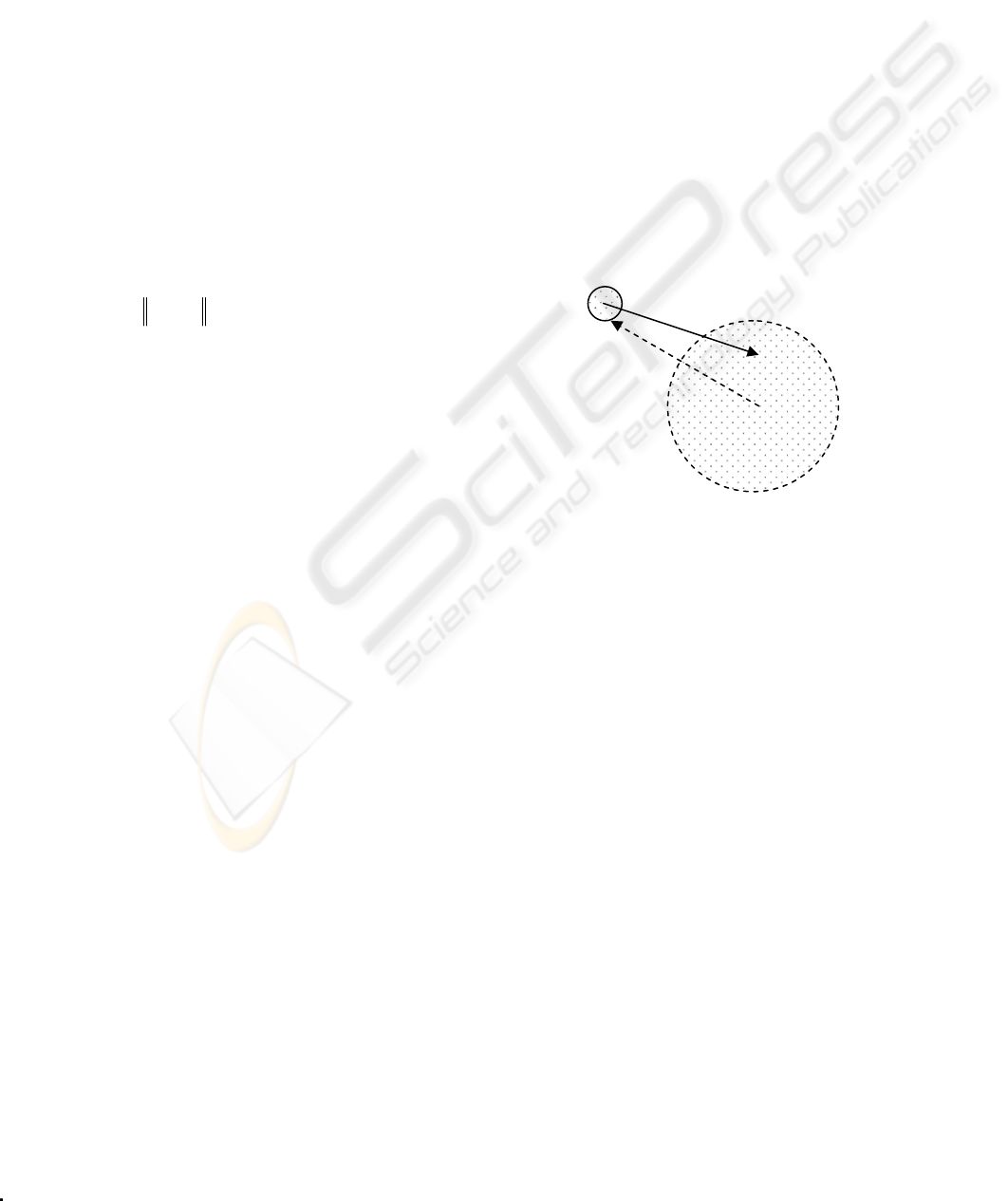
This can be demonstrated in Fig.2. If a point of set
A
has a larger divergence than the points of set
B as
illustrated in Fig.2, then, each point of its
neighbourhood in
A have similar divergence that are
more than divergences of the points of
B. Thus, the
control points will be selected from set
A rather than
set
B. It is clear that in this manner, the distribution
of the selected control points will not be uniform
over the original data point set. Therefore, it is
necessary to further require that each control point
should hold a large divergence with respect to all the
control points
BA∪ , so that the control points can
be distributed over the original data point set as
uniformly as possible. The divergence of each point
i
x is computed as follows,
⎪
⎪
⎩
⎪
⎪
⎨
⎧
⎟
⎟
⎠
⎞
⎜
⎜
⎝
⎛
−−=
⎟
⎟
⎠
⎞
⎜
⎜
⎝
⎛
−−=
∑
∑
∈
∈
0
))((2
))((1
S
T
iii
S
T
iii
trdiv
trdiv
y
x
xyxy
xxxx
, (7)
where,
S is the data point set while
0
S is the control
point set. The control point
c
x is selected using
(
)
ii
i
c
divdiv 21maxarg
+
=
x
, where arg(·) extracts
the point
i
x which yields the maximum of
(
)
ii
divdiv 21
+
.
Figure 2: The divergence of different point sets. The
points in A have a similar divergence that is larger than the
divergence of the points in B.
However, the implementation of Eq.(7) is time-
consuming. In practice, we prefer to use a standard
clustering algorithm (Duda et al. 2001) instead. For
clarity, some concepts need to be first defined as
follows.
z Centre of a partition
i
P is regarded as clustering
centre, which is defined as,
()()
0
)()()(
,,maxarg SPtr
ii
i
j
S
T
i
j
i
j
j
i
∈∈
⎟
⎟
⎠
⎞
⎜
⎜
⎝
⎛
−−=
∑
∈
yxxxxxy
x
;
z Measure between two points,
(
)
Strd
ji
T
jijiij
∈−−= xxxxxx ,,))(( ;
Based on the above definitions, our Partition
Algorithm can be stated as follows:
1)
{Clustering}
{Initializing}: Input data point set S, centre
set
0
S and an initial partition SP
i
r
i
=
=1
∪ ;
A
B
VISAPP 2006 - IMAGE UNDERSTANDING
176

{Merging, Splitting and Deleting}: These
standard clustering operations are carried out based
on the above definitions of the measure
ij
d and the
selected centre
0
S
i
∈y ;
Iteration until there is no change in each
i
P ;
2)
{Partitioning G}
Loop: from i=1 to r
Partition G in terms of
i
P ;
EndLoop;
The proposed partition algorithm is a divergence-
based iterative approach. The initial centre set
0
S is
usually the point set with the first r maximum
singular values of columns of G. The measure
between two points is indeed another representation
of the Euclidean distance. It can make the centers of
partitions as divergent as possible. But the clustering
algorithm is only an approximation of Eq.(7). Thus,
our partition algorithm can only approximate the
global optimal partition.
In short, the presented partition-based SVD
approach and partition algorithm constitute our
SVD-based approach for dataset simplification. It is
clear that data redundancy and computational
complexity of the large-sized range dataset can be
effectively amended in this SVD-based approach.
The highlight property of this approach is that the
control points are not fixed in advance. This means
that the basis functions can be modified adaptively
in terms of the change of range dataset. The
resulting solution of Eq.(2) would be a global least
square solution.
4 EXPERIMENTS AND
ANALYSIS
An intuitional way to evaluate the data point
simplification is to visualize the resulting implicit
surface. Our experiments of simplifying dataset are
first carried out on a range dataset of human faces
for a detailed analysis. The original range dataset
includes about 35,000 points, which is meshed and
illustrated in Fig.3a.
In the first experiment, we apply the pseudo-inverse
approach to this dataset. About 2,100 control points
are chosen uniformly over the whole dataset. The
resulting surface is shown in Fig.3b. Due to the
reduction of the control points, many details of the
face are lost. However, it can be noted that the
essential structures are preserved. Clearly, the
control points determine the essential structures of
the face in the resulting implicit surface. When the
control points are chosen uniformly over the whole
original dataset, the essential features can be
unbiasedly chosen as the control points. Indeed, the
influence of the non-control points in Eq.(5) is very
limited. We also show the resulting surface only
based on the control points in Fig.3c (i.e. non-
control points are not used). Obviously, the variance
between Fig.3b and Fig.3c is very small.
Furthermore, reducing the number of control points
to about 1,100, we fit the surface on the basis of a
selected control point set. The resulting surface is
shown in Fig.3d. It can be noted that there are no
distinct details lost in Fig.3d compared with Fig.3c.
This indicates that uniform sampling can preserve
the essential structures of the face. But it can also be
noted that distortions are also visible around the
nose in Fig.3d.
In the second experiment, we apply the SVD-based
approach to the same range dataset as in Fig.3a. In
this approach, the partition of G dominates the
quality of the resulting surface. Thus, the two
criteria of Eq.(7) become highlighted. In our
experiment, we first consider the first criterion of
Eq.(7), i.e.
⎟
⎟
⎠
⎞
⎜
⎜
⎝
⎛
−−=
∑
∈Sx
T
iii
trdiv ))((1 xxxx , as the
criterion of partition. Herein, the Partition Algorithm
described in section 3.2 is simply replaced by sorting
{
}
i
div1 . The control points are reduced to 30,000,
10,000 and 6,000 points respectively. The resulting
surfaces are shown in Fig.4. It can be noted that due
to the non-uniformity of the control points, many
structures are lost. Clearly, some regions contain few
or no control points (such as the nose area) while
others contain an excess of control points (such as
the cheek area). However, the essential facial
outlines are still retained. Moreover, when we
consider the two criteria of Eq.(7), i.e. use the
partition algorithm to obtain an appropriated
partition of G, it can be noted that some details of
the face can also be preserved even if the control
points are further reduced. The resulting surfaces
with the different numbers of control points are
shown in Fig.5.
Furthermore, comparing our SVD-Based Approach
with the uniformed down-sampling approach, we
can compare Fig.5c and Fig.5d with Fig.3c and
Fig.3d. This is because in Fig.3c and Fig.3d, we
uniformly down-sampled the control points over the
original range dataset, and the other non-control
points were discarded. In addition, the number of
control points in Fig.3c and Fig.3d are similar to the
number of control points in Fig.5c and Fig.5d
respectively. It can be noted that Fig.5c and Fig.5d
appear more distinct and preserve more details than
SIMPLIFIED REPRESENTATION OF LARGE RANGE DATASET
177
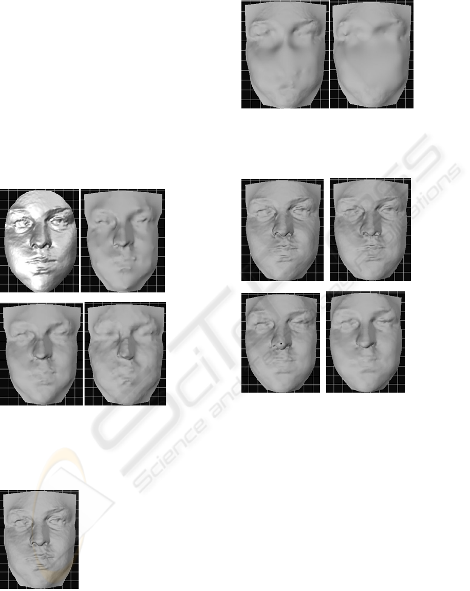
Fig.3c and Fig.3d, and there are comparatively less
distortions in Fig.5c and Fig.5d.
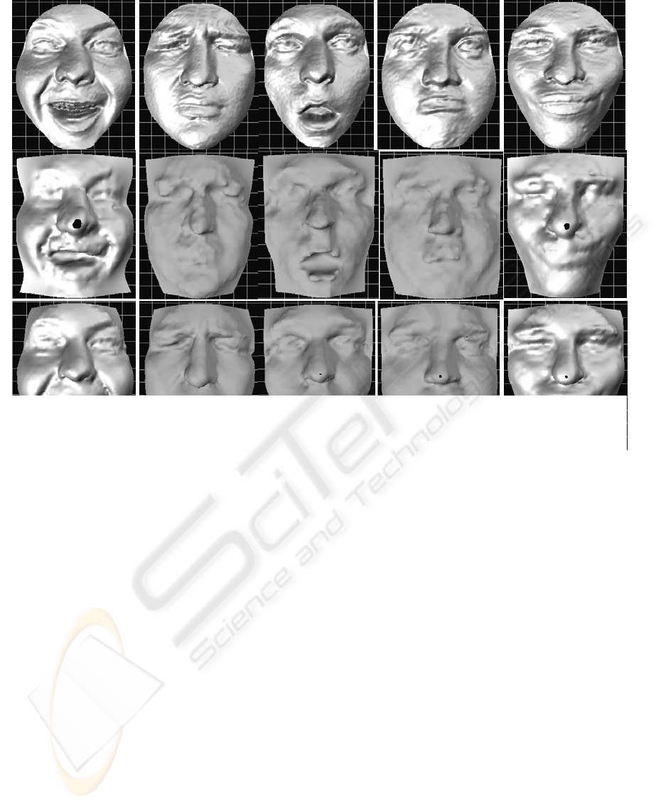
In order to further verify the efficiency of the SVD-
Based Approach, we subsequently apply the SVD-
Based Approach to 5 range datasets with different
facial expressions. The original numbers of data
points are in the range of 32,000-35,000, and are
reduced to 1,100 through our SVD-Based Approach.
For comparison, we also apply the uniform sampling
approach to these 5 range datasets, and their point
numbers are also reduced to about 1,100. All the
resulting surfaces are shown in Fig.6. It can be noted
that the resulting surfaces obtained by the SVD-
Based Approach preserve more details, and have
less distortions compared to the ones obtained by the
uniform sampling approach.
a. b.
c. d.
Figure 3: The resulting surfaces through the Pseudo-
Inverse Approach. a) original model, b) result using
pseudo-inverse approach, c) result using uniform sampling
approach, d) result using uniform down-sampling
approach, in which the number of points is reduced to
about 1,100.
a. 30,000 points
b. 10,000 points c. 6,000 points
Figure 4: The facial model is simplified by the SVD-based
approach with the first criterion of Eq.(7). Non-uniform
sampling leads to the quality of the resulting surfaces
decreasing quickly.
a. 10,000 points b. 6,000 points
c. 2,000 points d. 1,100 points
Figure 5: The facial model is simplified by the SVD-based
approach with the two criterion of Eq.(7). Considering the
uniform sampling preserves many details effectively.
5 CONCLUSIONS
In this paper, we presented two approaches of
computational simplification for medium- or large-
sized range dataset, one is the Pseudo-Inverse
Approach, and the other is the SVD-Based
Approach. The novelty in this paper is that we
devised a novel partition-based SVD algorithm,
which can effectively reduce the dimension of a
symmetric square matrix in a given partition case.
We combined the partition-based SVD algorithm
with a standard clustering algorithm to form our
SVD-Based Approach. Experimental results indicate
that in a given control point set case, the Pseudo-
Inverse Approach can give an optimal solution in a
least square sense. While in the case of an unknown
VISAPP 2006 - IMAGE UNDERSTANDING
178
control point, the SVD-Based Approach can seek an
appropriate control point set automatically, and the
resulting surface can preserve more details and
generate less distortions.
REFERENCES
Carr, J.C. and Beatson, R.K. et al., 2003. Smooth surface
reconstruction from noisy range data, ACM
GRAPHITE 2003, Melbourne, Australia, pp.119-126.
Carr, J.C. and Beatson, R.K. et al., 2001. Reconstruction
and Representation of 3D Objects with Radial Basis
Functions, ACM SIGGRAPH 2001, Los Angeles, CA,
pp.67-76.
Carr, J.C., Fright, W.R. and Beatson, R.K., 1997. Surface
Interpolation with Radial Basis Functions for Medical
Imaging, IEEE Transactions on Medical Imaging, Vol.
16, No. 1, pp.96-107.
Morse, B.S. and Yoo, T.S. et al., 2001. Interpolating
Implicit Surfaces from Scattered Surface Data Using
Compactly Supported Radial Basis Functions, in Proc.
of the Intel Conf on Shape Modeling & Applications,
pp.89-98.
Fleishman, S., Cohen-Or, D. and Silva, C.T., 2005. Robust
moving least-squares fitting with sharp features, ACM
Transactions on Graphics, Vol.24, Issue 3.
Beatson, R.K., Cherrie, J.B. and Mouat, C.T., 1999. Fast
fitting of radial basis functions: Methods based on
preconditioned GMRES iteration, Advances in
Computational Mathematics, Vol.11, pp.253–270.
Beatson, R.K., Cherrie, J.B. and Ragozin, D.L., 2001. Fast
evaluation of radial basis functions: Methods for four-
dimensional polyharmonic splines, SIAM J. Math.
Anal., Vol.32, No.6, pp.1272–1310.
Beatson, R.K., Light, W.A. and Billings, S., 2000. Fast
solution of the radial basis function interpolation
equations: Domain decomposition methods, SIAM J.
Sci. Comput., Vol.22, No.5, pp.1717–1740.
Suter, D., 1994. Fast evaluation of splines using poisson
formula. Intl. J. of Scientific Computing and
Modeling, Vol.1, No.1, pp.70–87.
Yu, H.C. and Bennamoun, M., 2005. Simplified
Representation of Large Range Dataset, Technical
Report, School of CSSE, Univ. of Western Australia.
Duda, R.O., Hart, P.E. and Stork, D.G., 2001. Pattern
Classification (2nd ed.), Wiley Interscience
.
SIMPLIFIED REPRESENTATION OF LARGE RANGE DATASET
179
