
STEREO VISION-BASED DETECTION OF MOVING OBJECTS
UNDER STRONG CAMERA MOTION
Hern
´
an Badino, Uwe Franke, Clemens Rabe, Stefan Gehrig
DaimlerChrysler AG
71059 Sindelfingen, Germany
Keywords:
Stereo Vision, Kalman Filter, Tracking, Ego-Motion Estimation
Abstract:
The visual perception of independent 3D motion from a moving observer is one of the most challenging
tasks in computer vision. This paper presents a powerful fusion of depth and motion information for image
sequences. For a large number of points, 3D position and 3D motion is simultaneously estimated by means of
Kalman Filters. The necessary ego-motion is computed based on the points that are identified as static points.
The result is a real-time system that is able to detect independently moving objects even if the own motion is
far from planar. The input provided by this system is suited to be used by high-level perception systems in
order to carry out cognitive processes such as autonomous navigation or collision avoidance.
1 INTRODUCTION
The visual perception of independent 3D motion from
a moving observer is one of the most challenging
tasks in computer vision. Independent 3D motion
is defined as the rigid or articulated change in po-
sition over time of an object with respect to an en-
vironment which is considered static. The percep-
tion of visual motion in animals and humans serves
a wide variety of crucial roles: ”way-finding (optic
flow), perception of shape from motion, depth segre-
gation, judgments of coincidence (time to collision,
time to filling a tea cup), judgments of motion direc-
tion and speed, and perception of animate, biologi-
cal activity” (Sekuler et al., 2004). In this paper we
present a passive approach for the simultaneous esti-
mation of position and velocity of single points, pro-
viding low-level information to more complex visual
perception systems, such as autonomous navigation
or collision avoidance. Treating such a process as a
low-level task should not be surprising since, from the
biological point of view, motion detection is a direct
experience uniquely specified by the visual system.
1
The further segmentation and integration of the infor-
1
Neurons in the middle temporal visual area integrate
motion signals over large regions of visual space and re-
spond to motion in their preferred direction, e.g. these neu-
rons register motion information per se. More advanced
perception activities are distributed over many areas of the
brain, each extracting somewhat different information from
mation provided by our approach is here referred to
as high-level vision, which must introduce some addi-
tional knowledge and intelligence to carry out a cog-
nitive process (”a bicyclist is approaching from the
left and we are going to collide with him within the
next two seconds”).
In order to estimate the velocity of a world point,
we must be able to observe its change of position over
time. The point position is easily obtained with multi-
ocular platforms
2
, which allow the instantaneous ex-
traction of 3D position through triangulation. The
time component is obtained by finding correspon-
dences in consecutive frames. The correspondences
are found between image points, i.e. optical flow
or normal flow, or at the level of objects, which re-
quires the previous segmentation of stereo points and
the further tracking of objects. This last approach
is commonly solved by an orthographical projection
of the 3D points into an evidence-grid-like structure
giving a bird-view of the scene, and grouping the
projections according to their vicinity (Martin and
Moravec, 1996). This method has its difficulties in
segmenting distant objects and in separating distinct
objects which are close together. The second op-
tion, i.e. normal flow, has some advantages with re-
the retinal image (Sekuler et al., 2004).
2
For the state-of-the-art on monocular methods see for
example (Kang et al., 2005), (Vidal, 2005) and (Woelk,
2004)
253
Badino H., Franke U., Rabe C. and Gehrig S. (2006).
STEREO VISION-BASED DETECTION OF MOVING OBJECTS UNDER STRONG CAMERA MOTION.
In Proceedings of the First International Conference on Computer Vision Theory and Applications, pages 253-260
DOI: 10.5220/0001375702530260
Copyright
c
SciTePress

spect to optical flow in the sense that it reduces the
correspondence problem (see for example (Argyros
and Orphanoudakis, 1997) and (Morency and Darrell,
2002)). Nevertheless, normal flow is less informative
compared to optical flow since it reflects only the mo-
tion in the direction of the image gradient and, there-
fore, does not provide an accurate estimation of point
motion.
Methods based on optical flow have been widely
proposed. One of the first attempts to fuse stereo
and optical flow information was studied by Wax-
man and Duncan in (Waxman and Duncan, 1986),
exploiting the relationship between 3D motion and
image velocities with stereo constraints. Kellman
and Kaiser (Kellman and Kaiser, 1995), Heinrich
(Heinrich, 2002) and Mills (Mills, 1997) also make
use of such constraints to detect independent mo-
tion. Demirdjian and Horaud (Demirdjian and Ho-
raud, 2000) propose a method for the estimation of
the ego-motion and the segmentation of moving ob-
jects. Demirdjian and Darrel (Demirdjian and Darrel,
2001) estimate rigid motion transformation mapping
two reconstructions of a rigid scene in the disparity
space (which they called d-motion). Dang et al (Dang
et al., 2002) fuse optical flow and stereo disparity us-
ing Kalman Filters for object tracking, where the de-
tection and segmentation of the object must have al-
ready been carried out. Kalman Filters were also used
by Zhang and Faugeras (Zhang and Faugeras, 1991)
for multiple motion estimation. Algorithms for the
detection of moving objects using dense stereo and
optical flow were proposed by Talukder and Matthies
(Talukder and Matthies, 2004) and by Agrawal et al
(Agrawal et al., 2005).
In this paper we describe an elegant approach
for the estimation and continuous refinement of the
position and velocity of world points. The six-
dimensional state (i.e. 3D position and 3D velocity)
as well as the six degrees of freedom (d.o.f.) of the
ego-motion (translation and rotation in 3D Euclidian
space) are estimated only based on the analysis of the
images provided by the cameras and the required cali-
bration parameters. Steps towards this approach have
been described in (Franke et al., 2005) where ego-
motion was restricted to a planar motion and obtained
with the inertial sensors of the vehicle. Our approach
combines binocular disparity and optical flow using
Kalman Filters (KF), providing an iterative refine-
ment of the 3D position and the 3D velocity of single
points. Ego-motion estimation is achieved by com-
puting the optimal rotation and translation between
the tracked static points of multiple frames. These
two processes are explained in detail in sections 2 and
3. In section 4 the whole algorithm is summarized.
In Section 5 we present experimental results with real
image sequences. In the last section we summarize
the paper.
2 ESTIMATION OF 3D POSITION
AND 3D VELOCITY
The main goal of our approach is the estimation of
position and velocity of world points in 3D Euclid-
ian space, and the recursively improvement of these
estimates over time. A continuous improvement of
the estimations is motivated by the noisy nature of
the measurements and, therefore, Kalman Filters are
the appropriate method to address this problem. In
this section we describe a model which estimates the
relative motion of world points relative to the ob-
server, compensating the ego-motion of the camera
platform with the observed motion of the points. If a
world point is static, its observed motion is described
as the inverse of the camera motion. Otherwise the
point presents an independent 3D motion which we
estimate. In the following subsections we assume a
vehicle-based coordinate system, i.e. the origin of the
coordinate system moves along with the observer.
2.1 Kalman Filter Model
Let suppose
x
k−1
=(X, Y, Z)
T
represents a world
point observed by the system at time t
k−1
and
v
k−1
=(
˙
X,
˙
Y,
˙
Z)
T
is its associated velocity vector.
As the camera platform moves in its environment, so
also does
x
and after a time ∆t
k
the new position of
the point in the vehicle coordinate system is given by:
x
k
=
ˆ
R
k
x
k−1
+
ˆ
d
k
+∆t
k
ˆ
R
k
v
k−1
(1)
where
ˆ
R
k
and
ˆ
d
k
, are the rotation matrix and transla-
tion vector of the scene, i.e. the inverse motion of the
camera. The velocity vector
v
k
, in vehicle coordinate
system, changes its direction according to:
v
k
=
ˆ
R
k
v
k−1
(2)
Combining position and velocity in the state vector
x
k
=(X, Y, Z,
˙
X,
˙
Y,
˙
Z)
T
leads to the discrete linear
system model equation:
x
k
= A
k
x
k−1
+ B
k
+ ω (3)
with the state transition matrix
A
k
=
ˆ
R
k
∆t
k
ˆ
R
k
0
ˆ
R
k
(4)
and the control matrix
B
k
=
⎡
⎢
⎢
⎣
ˆ
d
k
0
0
0
⎤
⎥
⎥
⎦
(5)
The noise term ω is assumed to be Gaussian white
noise with a covariance matrix Q.
VISAPP 2006 - MOTION, TRACKING AND STEREO VISION
254
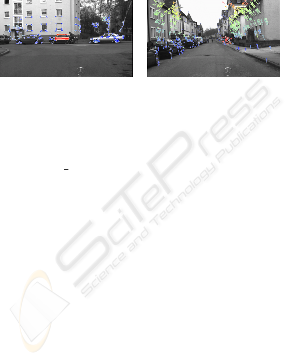
Figure 1: 3D motion vectors obtained when the vehicle
drives on a flat street. The inertial sensors of the vehicle
are used for the computation of the camera motion.
The measurement model captures the informa-
tion delivered by the stereo and optical flow sys-
tems. Assuming a pin-hole camera at the position
(0, height, 0)
T
in the vehicle coordinate system with
the optical axis parallel to the Z component, the non-
linear measurement equation for a point given in the
camera coordinate system is
z =
u
v
d
=
1
Z
Xf
u
Yf
v
bf
u
+ ν (6)
where (u, v) corresponds to the updated position of
the point obtained with the optical flow, d is the dis-
parity measured with stereo and (f
u
,f
v
) are the fo-
cal length in pixel width and height respectively. The
noise term ν is assumed to be Gaussian white noise
with a covariance matrix R.
This fusion of binocular disparity and optical flow
offers a powerful tool for the iterative estimation of
the position and velocity of world points. An exam-
ple is shown in figure 1. The arrows correspond to
the estimated direction. The warmth of the color en-
codes the 3D Euclidian velocity. Notice that the bi-
cyclist and the vehicle at the background are close to-
gether. Nevertheless a clear segmentation of both is
possible thanks to the additional information of ve-
locity. The rotation matrix and the translation vector
of equations 1 to 5 are normally obtained from the in-
ertial sensors of the vehicle which usually consist of
a speedometer and a yaw-rate sensor (Franke et al.,
2005). For indoor applications the information deliv-
ered by these inertial sensors is usually sufficient in
order to robustly estimate the position and velocity of
world points. However, for many other applications
(e.g. vehicle assistance systems) the motion of the
camera platform is not purely planar. Figure 2 shows
an example when the cameras are mounted in a vehi-
cle. It is obvious that the error in the velocity vectors
is produced by the roll rotation. A better approach is
possible if all six d.o.f. are considered computing the
ego-motion only from the images.
Figure 2: 3D motion vectors obtained when the vehicle
drives on an uneven street. Only yaw-rate and velocity are
considered in the ego-motion compensation.
3 ROBUST EGO-MOTION
ESTIMATION
Computing ego-motion from an image sequence
means obtaining the change of position and orienta-
tion of the observer with respect to a static scene,
i.e. the motion is relative to an environment which
is considered static. In most approaches this fact
is exploited and ego-motion is computed as the in-
verse of the scene motion (Demirdjian and Horaud,
2000), (Mallet et al., 2000), (Matthies and Shafer,
1987), (Olson et al., 2003), (van der M. et al., 2002),
(Badino, 2004). In the latter a robust approach for the
accurate estimation of the six d.o.f. of motion (three
components for translation and three for rotation) in
traffic situations is presented. In this approach, stereo
is computed at different times and clouds of 3D points
are obtained. The optical flow establishes the point-
to-point correspondence. The motion of the camera
is computed with a least-squares approach finding the
optimal rotation and translation between the clouds.
In order to avoid outliers, a smoothness motion con-
straint is applied rejecting all correspondences which
are inconsistent with the current motion. This last
two steps are also applied between non-consecutive
frames. In the next sub-sections we briefly review the
main steps of this approach.
3.1 Obtaining the Absolute
Orientation Between Two
Frames
Let X = {x
i
} be the set of 3D points of the pre-
vious frame and P = {p
i
} the set of 3D points ob-
served at the current frame, where x
i
↔ p
i
, i.e. p
i
is
the transformed version at time t
k
of the point x
i
at
time t
k−1
. In order to obtain the motion of the cam-
era between the current and the previous frame we
minimize a function which is expressed as the sum of
the weighted residual errors between the rotated and
STEREO VISION-BASED DETECTION OF MOVING OBJECTS UNDER STRONG CAMERA MOTION
255

translated data set X with the data set P , i.e.:
n
i=1
w
i
p
i
− R
k
x
i
−
d
k
2
(7)
where n is the amount of points in the sets, R
k
is
a rotation matrix,
d
k
is a translation vector, and w
i
are individual weights representing the expected er-
ror in the measurement of the points. To solve this
least-squares problem we use the method presented
by Horn (Horn, 1987), which provides a closed form
solution using unit quaternions. In this method the op-
timal rotation quaternion is obtained as the eigenvec-
tor corresponding to the largest positive eigenvalue of
a 4 × 4 matrix. The quaternion is then converted to
the rotation matrix. The translation is computed as
the difference of the centroid of data set P and the ro-
tated centroid of data set X. The computation of the
relative orientation is not constrained to this specific
method. Lorusso et al (Lorusso et al., 1995) shortly
describe and compare this and another three methods
for solving this problem in closed form.
3.2 Motion Representation with
Matrices
In order to simplify the notation of the following sub-
sections, we represent the motion in homogeneous co-
ordinates. The computed motion of the camera be-
tween two consecutive frames, i.e. from frame k − 1
to frame k, is represented by the matrix M
k
where:
M
k
=
R
k
d
k
01
(8)
The rotation matrix
ˆ
R
k
and translation vector
ˆ
d
k
from
equations 1 to 5 are obtained by just inverting M
k
,
i.e.:
M
−1
k
=
ˆ
R
k
ˆ
d
k
01
=
R
−1
k
−R
−1
k
d
k
01
(9)
The total motion of the camera since initialization can
be obtained as the products of the individual motion
matrices:
M
k
=
k
i=1
M
i
(10)
A sub-chain of movements from time t
n
to time t
m
is:
M
n,m
= M
−1
n
M
m
=
m
i=n+1
M
i
(11)
Figure 3 shows an example of motion integration with
matrices. As we will show later in section 3.4 equa-
tion 11 will support the integration of the motion be-
tween two non-consecutive frames (multi-step esti-
mation).
0
1
2
3
4
∏
=
−
==
∏
=
=
Figure 3: The integration of single-step estimations can be
obtained by just multiplying the individual motion matrices.
Every circle denotes the state (position and orientation) of
the camera between time t
0
and time t
4
. Vectors indicate
motion in 3D-space.
3.3 Smoothness Motion Constraint
Optical flow and/or stereo can deliver false informa-
tion about 3D position or image point correspondence
between image frames. Some of the points might also
correspond to an independently moving object. A ro-
bust method should still be able to give accurate re-
sults facing such situations. If the frame rate is high
enough in order to obtain a smooth motion between
consecutive frames, then the current motion is similar
to the immediate previous motion. Therefore, before
including the pair of points p
i
and x
i
into their corre-
sponding data sets P and X, we evaluate if the vec-
tor v
i
=
−−→
p
i
x
i
indicates a coherent movement. Let us
define m =[
˙x
max
˙y
max
˙z
max
1
] as the max-
imal accepted error of the position of a 3D point with
respect to a predicted position. Based on our previ-
ous ego-motion estimation step we evaluate the mo-
tion coherence of the vector v
i
as:
c
i
= M
k−1
x
i
− p
i
(12)
i.e. the error of our prediction. If the absolute value
of any component of c
i
is larger than m the pair of
points are discarded and not included in the data sets
for the posterior computation of relative orientation.
Otherwise we weight the pair of points as the ratio of
change with respect to the last motion:
w
i
=1−
c
i
2
m
2
(13)
which is later used in equation 7. Equations 12 and
13 define the smoothness motion constraint (SMC).
3.4 Multi-Frame Estimation
Single step estimation, i.e. the estimation of the mo-
tion parameters from the current and previous frame
is the standard case in most approaches. If we are
able to track points over m frames, then we can also
compute the motion between the current and the m
previous frames and integrate this motion into the
VISAPP 2006 - MOTION, TRACKING AND STEREO VISION
256

single step estimation (see figure 4). The estimation
of motion between frame m and the current frame k
(m<k−1) follows exactly the same procedure as ex-
plained above. Only when applying the SMC, a small
change takes place, since the prediction of the posi-
tion for k − m frames is not the same as for a single
step. In other words, the matrix M
k−1
of equation 12
is not valid any more. If the single step estimation for
the current frame was already computed as
˜
M
k
equa-
tion 12 becomes:
c
i
= M
−1
k−m
M
k−1
˜
M
k
x
i
− p
i
. (14)
Equation 14 represents the estimated motion between
times t
k−m
and t
k−1
(from equation 11), updated
with the current simple step estimation of time t
k
.
This allows the SMC to be even more precise, since
the uncertainty in the movement is now based on an
updated prediction. On the contrary in the single step
estimation, the uncertainty is based on a position de-
fined by the last motion.
Once the camera motion matrix
˜
M
m,k
between
times t
k−m
and t
k
is obtained, it is integrated with
the single step estimation. This is performed by an
interpolation. The interpolation of motion matrices
makes sense if they are estimations of the same mo-
tion. This is not the case since the single step motion
matrix is referred to as the motion between the last
two frames and the multi-step motion matrix as the
motion between m frames in the past to the current
one. Thus, the matrices to be interpolated are
˜
M
k
and
M
−1
m,k−1
˜
M
m,k
(see figure 4). The corresponding ro-
tation matrices are converted to quaternions in order
to apply a spherical linear interpolation. The interpo-
lated quaternion is converted to the final rotation ma-
trix R
k
. Translation vectors are linearly interpolated,
obtaining the new translation vector
t
k
. The factors
of the interpolation are given by the weighted sum of
the quadratic deviations obtained when computing the
relative motion of equation 7.
0
1
2
3
4
4
4
−
Figure 4: multi-frame approach. Circles represent the posi-
tion and orientation of the camera. Vectors indicate motion
in 3D-space.
˜
M
4
(single step estimation) and M
−1
1,3
˜
M
1,4
(multi-step estimation) are interpolated in order to obtain
the final estimation M
4
.
The multi-frame approach performs better thanks
to the integration of more measurements. It also re-
duces the integration of the errors produced by the
single-step estimation between the considered time
points. In fact, our experience has shown that without
the multi-frame approach the estimation degenerates
quickly and, normally, after a few hundred frames the
ego-position diverges dramatically from the true solu-
tion. Thus, the multi-frame approach provides addi-
tional stability to the estimation process.
4 THE ALGORITHM
This section summarizes the main tasks of our ap-
proach. 1. Left and Right Image Acquisition.
2. Measurement.
a. Compute optical flow (tracking).
b. Compute stereo disparity.
3. Ego-Motion Computation.
a. Apply SMC Single Step.
b. Compute Single Step (SS) estimation.
c. Apply SMC Multi-Step.
d. Compute Multi-Step (MS) estimation.
e. Interpolate SS and MS results.
4. Kalman Filter.
a. Compute A and B matrices with ego-motion
estimation (Step 3).
b. Update models.
5. Go to Step 1.
5 EXPERIMENTAL RESULTS
Our current implementation tracks 1200 points. It
runs at 12 − 16 Hz on a 3.2 GHz PC. We use a
speed-optimized version of the KLT algorithm (Shi
and Tomasi, 1994) and compute stereo using a coarse
to fine correlation method as described in (Franke,
2000). In order to show the robustness of the method,
we demonstrate the performance on three real world
sequences.
Uneven Street. In this sequence, the vehicle drives
on a slightly uneven street. A bicyclist appears sud-
denly from a back street at the right. The sequence has
200 stereo image pairs and was taken at 16 Hz. The
baseline of the stereo system is 0.35 meters and the
images have a VGA resolution. The car starts from a
standing position and accelerates up to a velocity of
30 km/h.
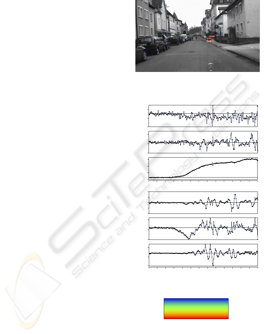
Figure 5(a) shows the improved results for the es-
timation already illustrated in figure 2. Thanks to the
ego-motion estimation, the artefacts disappear and the
bicyclist is clearly visible now. Figure 5(b) shows the
ego-motion estimation results for every frame of the
sequence. The minimum in the roll rotation at frame
120 correspond to the same frame number as above.
Notice that the lateral translation decreases together
with the velocity despite the small yaw rotation. This
STEREO VISION-BASED DETECTION OF MOVING OBJECTS UNDER STRONG CAMERA MOTION
257
indicates that the optical axis of the camera is not
aligned with the driving direction of the vehicle, i.e.
the camera is fixed mounted on the vehicle but view-
ing slightly to the right.
This last observation reveals another advantage of
computing the ego-motion directly from the images:
there is no need of an external calibration of the cam-
era platform w.r.t. the vehicle. Figure 6(a) shows the
velocity vectors for frame 146, using only inertial sen-
sors when the yaw rotation of the camera w.r.t. the
vehicle was wrongly estimated by 5 degrees. Figure
6(b) shows the results for the same camera configura-
tion using only ego-motion estimation.
Crossing Traffic with Background Occlusion.
Figure 7 shows the estimation results with an oncom-
ing bus. In this sequence, both the ego-vehicle and the
bus are driving in a curve. In the worst case, the bus
takes up more than 35% of the image area. The com-
putation of ego-motion is still possible here thanks to
the smoothness motion constraint, which selects only
static points (blue points in the image) for the ego-
motion computation.
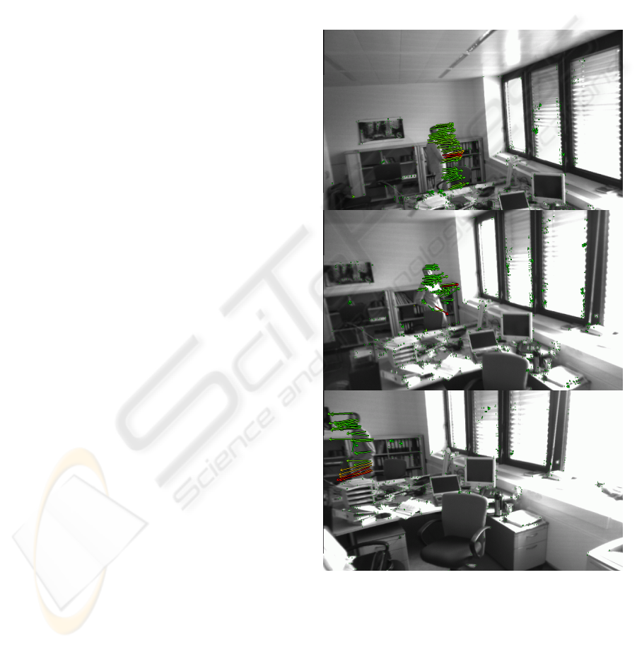
Indoor Environment. Figure 8 shows an example
of the results in an indoor environment. The sequence
shows a person walking behind a desktop while the
camera is translated and rotated by hand. The color
encoding is the same as in the two previous examples
but red now means 1.75 m/s. The different colors
of the arrows on the moving person correspond to the
different velocities of the different body parts (arms,
body and legs).
6 SUMMARY
We have presented a method for the efficient estima-
tion of position and velocity of tracked image points,
and for the iterative improvements of these estimates
over time. The scene structure is obtained with a
binocular platform. Optical flow delivers the change
of this structure in consecutive frames. By observ-
ing the dynamics of the individual 3D points, an es-
timation of their velocity is possible. This way we
obtain a six dimensional state for every world point
which is given in a vehicle coordinate system. As the
camera moves, the state of every point needs to be
updated according to the motion of the observer and,
therefore, the ego-motion of the cameras needs to be
known. Instead of obtaining motion information from
the error-prone inertial sensors of the vehicle, the six
d.o.f. of ego-motion are obtained as the optimal rota-
tion and translation between the current and previous
set of static 3D points of the environment. All this
information is fused using Kalman Filters, obtaining
an iterative improvement over time of the 3D point
position and velocity.
(a) 3D motion vectors. The arrows correspond to the esti-
mated 3D position of the points in 0.5 seconds back projected
into the image. The color encodes the velocity as shown in
image (c)
-0.023
-0.008
0.007
-0.017
-0.002
0.013
-0.050
0.130
0.310
0.490
-0.600
-0.300
0.000
0.300
0.600
-0.120
-0.020
0.080
-0.700
-0.200
0.300
5 20 35 50 65 80 95 110 125 140 155 170 185 200
5 20 35 50 65 80 95 110 125 140 155 170 185 200
M e t e r s
D e g r e e s
(b) Ego-motion estimation. The plots show the observed mo-
tion between consecutive frames. From top to bottom: X, Y ,
Z translations; pitch, yaw, roll rotations.
2 . 2 5 m / s
0 m / s
4 . 5 m / s
2 . 2 5 m / s
0 m / s
4 . 5 m / s
(c)
Figure 5: a bicyclist approaches from the right while the
vehicle drives on an uneven street.
This algorithm turned out to be powerful for the
detection of moving obstacles in traffic scenes. How-
ever, it is not limited to this application but may be
VISAPP 2006 - MOTION, TRACKING AND STEREO VISION
258

(a) 3D motion vectors using inertial sensors.
(b) 3D motion vectors estimating the six d.o.f. of motion.
Figure 6: results when the camera orientation was wrong
estimated. The images shows the state of the scene 1.5 sec-
onds later as in figure 5.
also useful for other applications such as autonomous
navigation, simultaneous localization and mapping or
target detection for military purposes.
REFERENCES
Agrawal, M., Konolige, K., and Iocchi, L. (2005). Real-
time detection of independent motion using stereo.
In IEEE Workshop on Motion and Video Comput-
ing (WACV/MOTION 2005), pages 672–677, Breck-
enridge, CO, USA.
Argyros, A. A. and Orphanoudakis, S. C. (1997). Indepen-
dent 3d motion detection based on depth elimination
in normal flow fields. In Proceedings of the 1997 Con-
ference on Computer Vision and Pattern Recognition
(CVPR ’97), pages 672–677.
Badino, H. (2004). A robust approach for ego-motion esti-
mation using a mobile stereo platform. In 1
st
Inter-
national Workshop on Complex Motion (IWCM’04),
G
¨
unzgburg, Germany. Springer.
Dang, T., Hoffmann, C., and Stiller, C. (2002). Fusing
optical flow and stereo disparity for object tracking.
In Proceedings of the IEEE V. International Con-
ference on Intelligent Transportation Systems, pages
112–117, Singapore.
Demirdjian, D. and Darrel, T. (2001). Motion estimation
Figure 7: estimation results when the moving objects takes
up a large area of the image. The time between the images
is 0.5 seconds.
from disparity images. In Technical Report AI Memo
2001-009, MIT Artificial Intelligence Laboratory.
Demirdjian, D. and Horaud, R. (2000). Motion-egomotion
discrimination and motion segmentation from image
pair streams. In Computer Vision and Image Under-
standing, volume 78(1), pages 53–68.
Franke, U. (2000). Real-time stereo vision for urban traffic
scene understanding. In IEEE Conference on Intelli-
gent Vehicles, Dearborn.
Franke, U., Rabe, C., Badino, H., and Gehrig, S. (2005).
6d-vision: Fusion of stereo and motion for robust en-
vironment perception. In DAGM ’05, Vienna.
Heinrich, S. (2002). Fast obstacle detection using
flow/detph constraint. In IEEE Intelligent Vehicle
Symposium (IV’2002), Versailles, France.
Horn, B. K. P. (1987). Closed-form solution of absolute ori-
entation using unit quaternions. In Journal of the Op-
STEREO VISION-BASED DETECTION OF MOVING OBJECTS UNDER STRONG CAMERA MOTION
259
tical Society of America A, volume 4(4), pages 629–
642.
Kang, J., Cohen, I., Medioni, G., and Yuan, C. (2005). De-
tection and tracking of moving objects from a moving
platform in presence of strong parallax. In IEEE In-
ternational Conference on Computer Vision ICCV‘05.
Kellman, P. J. and Kaiser, M. (1995). Extracting object mo-
tion during observer motion: Combining constraints
from optic flow and binocular disparity. JOSA-A,
12(3):623–625.
Lorusso, A., Eggert, D., and Fisher, R. B. (1995). A com-
parison of four algorithms for estimating 3-d rigid
transformations. In Proc. British Machine Vision Con-
ference, Birmingham.
Mallet, A., Lacroix, S., and Gallo, L. (2000). Position es-
timation in outdoor environments using pixel tracking
and stereovision. In Proceedings of the 2000 IEEE In-
ternational Conference on Robotics and Automation,
pages 3519–3524, San Francisco.
Martin, M. and Moravec, H. (1996). Robot evidence grids.
The Robotics Institute Carnegie Mellon University
(CMU-RI-TR-96-06).
Matthies, L. and Shafer, S. A. (1987). Error modeling in
stereo navigation. In IEEE Journal of Robotics and
Automation, volume RA-3(3), pages 239–248.
Mills, S. (1997). Stereo-motion analysis of image se-
quences. In Proceedings of the first joint Australia and
New Zealand conference on Digital Image and Vision
Computing: Techniques and Applications, DICTA’97
/ IVCNZ’97, Albany, Auckland, NZ.
Morency, L. P. and Darrell, T. (2002). Stereo tracking us-
ing icp and normal flow constraint. In Proceedings
of International Conference on Pattern Recognition,
Quebec.
Olson, C. F., Matthies, L. H., Schoppers, M., and Maimone,
M. W. (2003). Rover navigation using stereo ego-
motion. In Robotics and Autonomous Systems, vol-
ume 43(4), pages 215–229.
Sekuler, R., Watamaniuk, S. N. J., and Blake, R. (2004).
Stevens’ Handbook of Experimental Psychology, vol-
ume 1, Sensation and Perception, chapter 4, Percep-
tion of Visual Motion. Wiley, 3
rd
edition.
Shi, J. and Tomasi, C. (1994). Good features to track.
In IEEE Conference on Computer Vision and Pattern
Recognition (CVPR’94).
Talukder, A. and Matthies, L. (2004). Real-time detection
of moving objects from moving vehicles using dense
stereo and optical flow. In Proceedings of the IEEE In-
ternational Conference on Intelligent Robots and Sys-
tems, pages 315–320, Sendai, Japan.
van der M., W., Fontijne, D., Dorst, L., and Groen, F. C. A.
(2002). Vehicle ego-motion estimation with geomet-
ric algebra. In Proceedings IEEE Intelligent Vehicle
Symposium, Versialles, France, May 18-20 2002.
Vidal, R. (2005). Multi-subspace methods for motion
segmentation from affine, perspective and central
panoramic cameras. IEEE International Conference
on Robotis and Automation.
Waxman, A. M. and Duncan, J. H. (1986). Binocular im-
age flows: Steps toward stereo-motion fusion. PAMI,
8(6):715–729.
Woelk, F. (2004). Robust monocular detection of inde-
pendent motion by a moving observer. In 1
st
Inter-
national Workshop on Complex Motion (IWCM’04),
G
¨
unzgburg, Germany. Springer.
Zhang, Z. and Faugeras, O. D. (1991). Three-dimensional
motion computation and object segmentation in a long
sequence of stereo images. Technical Report RR-
1438, Inria.
Figure 8: a person moves first to the right (first image), turn
around (second image) and finally walk to the left (third
image) while the camera is translated and rotated with the
hand.
VISAPP 2006 - MOTION, TRACKING AND STEREO VISION
260
