
IMPROVED SEGMENTATION OF MR BRAIN IMAGES
INCLUDING BIAS FIELD CORRECTION BASED ON 3D-CSC*
Haojun Wang, Patrick Sturm, Frank Schmitt, Lutz Priese
Institute for Computational Visualistics, University of Koblenz-Landau, 56070 Koblenz, Germany
Keywords: Image segmentation, 3D Cell Structure Code, MRI, Brain, Classification.
Abstract: The 3D Cell Structure Code (3D-CSC) is a fast region growing technique. However, directly adapted for
segmentation of magnetic resonance (MR) brain images it has some limitations due to the variability of
brain anatomical structure and the degradation of MR images by intensity inhomogeneities and noise. In this
paper an improved approach is proposed. It starts with a preprocessing step which contains a 3D Kuwahara
filter to reduce noise and a bias correction method to compensate intensity inhomogeneities. Next the 3D-
CSC is applied, where a required similarity threshold is chosen automatically. In order to recognize gray
and white matter, a histogram-based classification is applied. Morphological operations are used to break
small bridges connecting gray value similar non-brain tissues with the gray matter. 8 real and 10 simulated
T1-weighted MR images were evaluated to validate the performance of our method.
1 INTRODUCTION
Segmentation of 3D MR brain images is an
important procedure for 3D visualization of brain
structures and quantitative analysis of differences
between normal and abnormal brain tissues. Up to
now many segmentation techniques have been
developed (Suzuk 1991,
MacDonald 2000, Zhang
2001, Stokking 2000, Schnack 2001). However,
most intensity-based schemes fail to segment MR
brain images into gray and white matter
satisfactorily due to the effect of intensity
inhomogeneities (also referred as bias field)
(Rajapakse 1998, Wells III 1996, Sled 1998)
resulting from irregularities of the scanner magnetic
fields, radio frequency, etc. The deformable-based
techniques sometimes do not converge well to the
boundary of interest due to the complicated
deformations in the anatomy (Pham 2000).
Furthermore existing fully automatic segmentation
techniques have to make a compromise between
speed and accuracy of processes in practice.
Therefore, an automatic robust and fast 3D brain
segmentation method is needed that is able to detect
gray and white matter.
*This work was supported by the BMBF under grant
01/IRC01B (research project 3D-RETISEG)
A 3D hierarchical inherently parallel region
growing method, called 3D-CSC, has recently been
developed in our group and at Research Centre
Juelich. It is an effective 3D generalization of the
2D-CSC (Priese 2005). In comparison with
traditional region growing techniques it does not
depend on the selection of seed points. It is very fast
due to its hierarchical structure. The advantages of
the technique are local simplicity and global
robustness. Therefore, we adapt the 3D-CSC for
segmentation of 3D MR brain images. In the 3D-
CSC, region growing is steered by a hierarchical
structure of overlapping cells. Overlapping and gray-
similar regions in one hierarchy level are merged to
a new region of the next level. Unfortunately some
known difficulties in MR brain images, such as
intensity inhomogeneities and the effect of noise,
degrade the performance of 3D-CSC segmentation.
This results in an over-segmentation. In order to
overcome these difficulties, a preprocessing step
which includes a 3D Kuwahara filter to reduce
random noise and a correction of intensity
inhomogeneities is applied. In addition, a
postprocessing step based on histogram-based
classification of CSC segments and morphology-
based shape constraints is integrated in our scheme.
All processing steps are fully automatic.
The paper is organized as follows: Section 2
briefly introduces 3D-CSC segmentation. Section 3
338
Wang H., Sturm P., Schmitt F. and Priese L. (2006).
IMPROVED SEGMENTATION OF MR BRAIN IMAGES INCLUDING BIAS FIELD CORRECTION BASED ON 3D-CSC.
In Proceedings of the First International Conference on Computer Vision Theory and Applications, pages 338-345
DOI: 10.5220/0001376503380345
Copyright
c
SciTePress
describes the improved segmentation scheme for
brain images. Experimental results and conclusion
are given in Section 4 and Section 5 respectively.
2 3D CELL STRUCTURE CODE
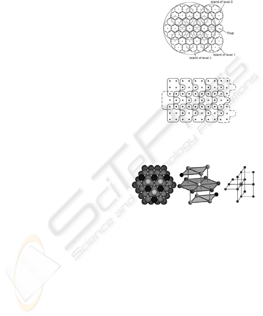
The 3D-CSC steers a hierarchical region growing on
a special 3D topology. In order to understand this
hierarchy we first introduce the hierarchical
hexagonal topology (see Figure 1(a)) of the 2D–CSC
(Rehrmann 1998). The topology is formed by so
called islands in different levels. An island of level 0
consists of a center pixel and its six neighboring
pixels. An island of level n+1 consists of a center
island of level n and its six neighboring islands of
level n. Two neighboring islands of level n overlap
in a common island of level n-1. This is repeated
until one big island covers the whole image. In order
to apply the hierarchical topology in a real image,
the hexagonal island structure is transformed
logically to an orthogonal grid as shown in Figure
1(b).
Generalizing the 2D hierarchical hexagonal
topology to 3D forms the 3D hierarchical cell
topology. It is constructed by the densest sphere
packing (see Figure 2(a)). Here we just focus on the
S
15
cell structure (see Figure 2(b) and 2(c) where
2(c) is a transformation into the orthogonal 3D
grid.). In S
15
a cell of level 0 consists of 15 voxels (1
center voxel and its 14 neighboring voxels).
The S
15
cell structure possesses the following
properties:
14-neighborhood: each cell of level n overlaps
with 14 cells of level n.
Plainness: two cells of level n+1 overlap each
other in at most one cell of level n.
Coverability: each cell (except the topmost one) of
level n is a sub-cell of a parent cell of level n+1.
Strong Saturation: all sub-cells (except the center
cell) of a cell of level n+1 are sub-cells of exactly
two different cells of level n+1. Each center cell
has exactly one parent cell.
These properties lead to a nice and efficient
implementation. Also the information about location
and neighborhood of each cell can be derived
quickly. In the 3D-CSC, region growing is done
independently in each cell of each level.
Neighboring and similar segments in lower levels
will be merged to bigger segments in a higher level.
If two neighboring segments are dissimilar they
will be split. For a deeper discussion see (Sturm
2004). Here ‘similar’ means the difference of the
mean intensity of two neighboring segments is
below a certain threshold T. The threshold T will be
chosen automatically.
(a)
(b)
Figure 1: The hierarchical hexagonal island structure and
its deformation on the orthogonal grid.
(a) (b) (c)
Figure 2: 3D hierarchical cell topology and S
15
cell
structure.
3 ADAPTION TO BRAIN IMAGES
The segmentation procedure for 3D MR brain
images consists of three parts:
Preprocessing: noise suppression and bias field
correction. (Described in section 3.1)
3D-CSC segmentation. (General case described in
section 2, adaption to MR brain images described
in section 3.3)
Postprocessing: classifying the primitive CSC
segments into brain and non–brain tissues, then
breaking small connections between them and
separating brain tissue into gray and white matter.
(Described in section 3.4)
IMPROVED SEGMENTATION OF MR BRAIN IMAGES INCLUDING BIAS FIELD CORRECTION BASED ON
3D-CSC
339
3.1 Preprocessing: Filter and Bias
Field Correction
To reduce noise, we apply a 3D generalization of the
Kuwahara filter as it gives a very good tradeoff
between performance and speed and has been
proved to be an ideal nonlinear filter for smoothing
regions and preserving edges (Kuwahara 1976).
Recently a successful method for dealing with
the bias field problem has been proposed (Vovk
2004). The idea behind it is to iteratively sharpen
probability distributions of image features along
intensity features by an intensity correction force.
Then the bias correction estimation is calculated.
This correction method combines intensity and
spatial information and estimates the intensity
inhomogeneity on each image point.
The following notations are given:
V is the number of voxels in an image
x
is the three dimensional location of a voxel
)(xu is the measured gray value at the location
x
in a MR image
)(xv is the ideal gray value in the absence of any
bias field
)(xn is noise at location
x
)(xf is the bias field at
x
)(uLd
u
= is the Laplacian (2
nd
derivative) of u
u
P is the probability distribution (2 dim.
histogram) of u and
u
d , where nbaP
u
=
),( tells
that exactly n voxels x
1
…,x
n
have the values
axu
i
=)( and bxd
iu
=)(
F
µ
is the mean value of the set of the absolute
force
F
(Vovk 2004) considers the usual model of image
formation in MR as:
)()()()( xnxfxvxu +
⋅
= (1)
)(xn is neglectable as we have already applied a
Kuwahara filter to reduce noise. First set
uu
=
:
1
,
then apply the following iteration (2)-(4):
)(ln
1
i
ui
P
a
V
F
∂
∂
⋅=
(2)
i
F are the correction forces and are derived by the
weighted partial derivate of logarithm of
i
u
P
along
the intensity value a (the first coordinate of
i
u
P
),
then are mapped to the points with corresponding
features in the image.
)(1
1
i
F
i
FG
k
f
i
⋅+=
−
µ
(3)
where G is a three dimensional Gaussian filter and
carries out a convolution with
i
F , k is a pre-chosen
parameter.
In the principle, the corrected image
i
v at iteration
i and the input image
1+i
u at iteration 1
+
i are
expressed as:
∏
=
−
−
+
⋅=⋅==
i
j
jiiii
fufuvu
1
1
1
1
(4)
However in practice, preserving the brightness of
the original input image
u must be taken into
account in each iterative correction (More details are
described in (Vovk 2004)). No automatic
termination criterion for the iterations is proposed in
(Vovk 2004). Hence we focus on this and consider
the mean of absolute variation
i
D (see equation (6))
which reflects the changes between the overall
estimated bias correction
1
ˆ
−
i
f after iteration i and
the initial correction
1
ˆ
1
0
=
−
f .
11
1
1
11
ˆˆ
**
−−
−
=
−−
⋅⋅≈⋅=
∏
ii
u
u
i
j
j
u
u
i
ffff
ii
µ
µ
µ
µ
(5)
1
0
1
ˆˆ
−−
−
=
ff
i
i
D
µ
(6)
In (5),
1
ˆ
−
i
f will be used to correct the original
input image
u , then the corrected image
i
v is
derived,
µ
is the mean value,
*
i
u is expressed by:
11
1
*
ˆ
−−
−
⋅⋅=
iii
ffuu (7)
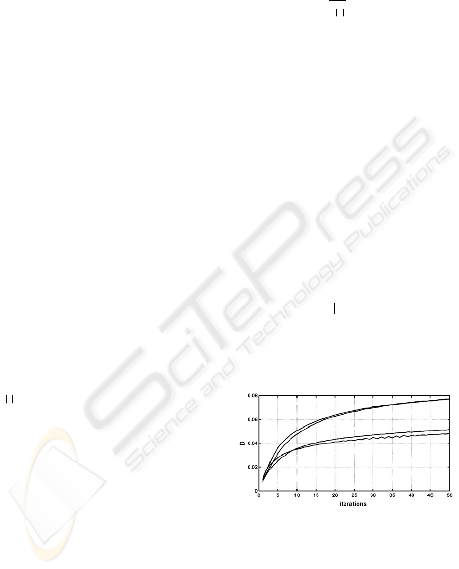
Figure 3:
i
D
fD(
curves for several tested images.
Figure 3 shows several typical curves of
i
D for
tested images.
i
D increases and tends to roughly
converge, although some small vibrations exist
locally. Images with low inhomogeneities converge
faster than those with high inhomogeneities. This
means images with low inhomogeneities need less
iterations for the correction. Thus a termination
VISAPP 2006 - IMAGE ANALYSIS
340
criterion will be derived, i.e. in each 5 iterations we
compute the regressive straight line of
i
D , if the
slope coefficient of the regressive straight line is
below a termination threshold E the iteration will
stop otherwise continue. The purpose of the
regressive straight line is to eliminate the effect of
small local vibrations of
i
D . This has been proved
to be robust in our tested images. With the same
constraint E the iterative corrections of all tested
images will stop after 10-25 steps according to their
degree of inhomogeneity .
To reduce computational cost for the Gaussian
convolution in equation (3), the MR data is down-
sampled by factor 3 in each dimension. The
degradation of performance is neglectable, because
the bias field varies just slowly across an image.
As the background is not degraded by the bias
field and could interfere with the estimation, it is
removed prior to our correction method
automatically.
3.2 Histogram Analysis
Histogram analysis plays an important role in our
method: We use it to detect the similarity threshold
for 3D-CSC segmentation and for classification after
the CSC. Image histograms contain information
about intensity distributions of tissues in MR
images. We here only consider T1 weighted MR
brain images. The histograms of those images
normally contain five modes, listed from dark to
bright: background, cerebrospinal fluid (CSF), gray
matter (GM), white matter (WM) and fat. The
spatial variations of the same tissue class and the
effect of bias field make them overlap each other.
After bias field correction the overlapping between
classes is reduced. This enables us to recognize them
in intensity space, i.e. to find thresholds that separate
those classes by their intensities.
First we consider the intensity histogram
h of
the preprocessed image as a Gaussian mixture model
(GMM) (see (8)-(9)), where each Gaussian
represents the intensity distribution of each tissue
class in an MR image. The approximated normalized
histogram
h
ˆ
is expressed by:
∑
=
⋅=
C
i
i
ii
Gah
1
ˆ
,
ˆ
ˆ
ˆ
σµ
(8)
C is the number of Gaussians,
i
a
ˆ
,
i
µ
ˆ
and
i
σ
ˆ
are the
estimated mixing weight, mean and standard
deviation of the i-th Gaussian which is given by:
(9)
where
g
is a gray level.
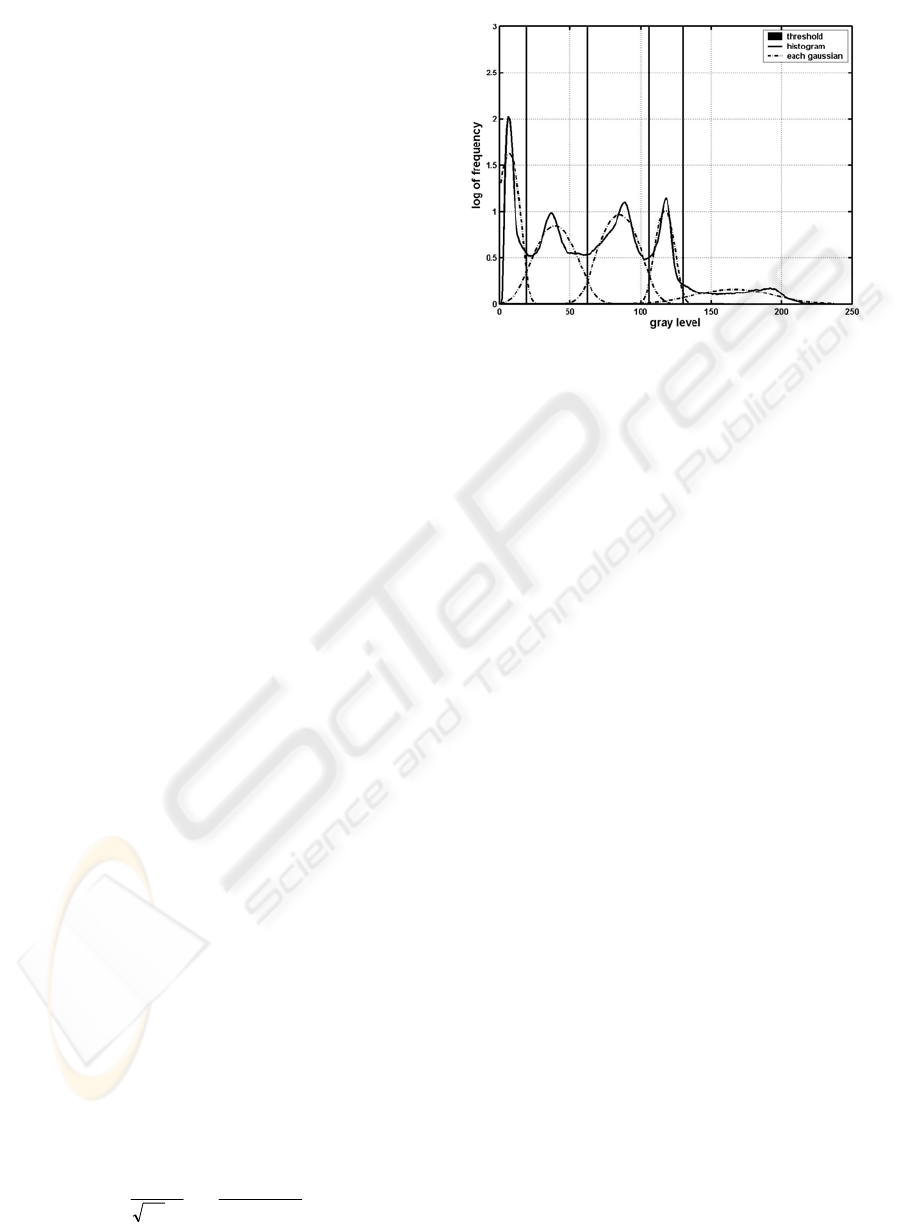
Figure 4: The result of histogram analysis.
To obtain the parameters of the Gaussian mixture
model we follow the scale space filtering method of
(Carlotto 1987). This gives us a good initialization
for
i
a
ˆ
,
i
µ
ˆ
, and
i
σ
ˆ
. With the Expectation-Maxi-
mization (EM) algorithm (Duda 2001), those
parameters are further refined.
The result of the GMM estimation for a sample
image and the thresholds separating the five classes
for later classification are shown in Figure 4 where
each Gaussian contains the mixing weight. We refer
to the threshold between background and CSF as t1,
between CSF and gray matter as t2, between gray
and white matter as t3 and between white matter and
fat as t4.
3.3 Adaption of the 3D-CSC for MR
Brain Images
As mentioned in section 2, the 3D-CSC requires a
similarity threshold T. As there is no constant value
for T applicable for all MR images, we developed an
automatic method for finding a reasonable value
based on the histogram analysis method described in
section 3.2. T is derived by computing the shortest
distance D
s
between the centers of two estimated
Gaussians in the histogram of the corrected image. T
is equal to D
s
divided by 4 which proved to result in
near-optimal values for MR brain images from
various sources.
3.4 Postprocessing
The 3D-CSC segmentation does not result in a
single segment for gray resp. white matter. Instead
gray and white matter are oversegmented and
⎥
⎥
⎦
⎤
⎢
⎢
⎣
⎡
⋅
−−
=
2
2
ˆ
,
ˆ
ˆ
2
)
ˆ
(
exp
ˆ
2
1
)(
i
ii
i
i
g
gG
σ
µ
σπ
σµ
t1
t2
t3 t4
background
CSF
fat
WM
GM
IMPROVED SEGMENTATION OF MR BRAIN IMAGES INCLUDING BIAS FIELD CORRECTION BASED ON
3D-CSC
341

sometimes parts of gray matter and non-brain tissues
are merged to one segment due to narrow gray value
bridges. Therefore some postprocessing steps are
needed: First the CSC segments are preliminary
classified in brain and non-brain by their mean gray
value (see 3.4.1). As only the mean gray value is
considered segments containing non-brain tissues
with an intensity similar to gray or white matter are
classified always as brain. This problem is solved by
morphological operations (see 3.4.2). Finally the
brain is separated into gray and white matter.
3.4.1 Preliminary Classification
We obtain a preliminary brain mask by doing a
classification of CSC segments in which we use the
intensity thresholds (see section 3.2) to select all
segments which could belong to the brain. I.e. if the
mean intensity of a segment belongs to the range [t2,
t4] the segment should be kept in the preliminary
brain mask otherwise discarded. However, even if
optimal thresholds are used, connections between
the brain and surrounding non-brain tissues still
occur. In order to break these connections and
reduce misclassification, morphological operations
are applied.
3.4.2 Morphological Operations and Final
Classification
We apply the following morphological operations to
break up bridges between brain and non-brain
tissues:
Select the largest connected component (LCC1) in
the preliminary brain mask and perform an erosion
with a ball structuring element with radius of 3-5
voxels (depending on the size of the input image).
This breaks connections between the brain and
non-brain tissues.
Select the largest connected component (LCC2)
after the erosion and perform a dilation with the
same size structuring element to get LCC3. This
reconstructs the eroded brain segment.
Compute the geodesic distances to LCC3 from all
points which only belong to LCC1 but not to
LCC3 using a 1 voxel radius ball structuring
element. Then assign all points whose distances
are <= 4 voxels to LCC3 as the final segmented
brain. In this step some more detailed structures of
the segmented brain are recovered
At last, we remove all voxels not belonging to
the brain mask from the CSC segments. The
threshold t3 is then applied to classify the remaining
segments into gray matter (GM) and white matter
(WM).
4 EXPERIMENTS AND RESULTS
To assess the performance of the proposed method,
we applied it to 18 T1-weighted MR brain images
(10 simulated images and 8 real images). The
simulated images were downloaded from the
Brainweb site (http://www.bic.mni.mcgill.ca/
brainweb). These images consist of 181x217x181
voxels sized 1x1x1mm with a gray value depth of 8
bits. 1%, 3%, 5%, 7% resp. 9% noise levels have
been added and intensity inhomogeneity levels
(“RF”) are 20% and 40%. The real images were
acquired at 1.5 Tesla with an AVANTO SIEMENS
scanner from the BWZK hospital in Koblenz,
Germany. They consist of 384x512x192 voxels
with 12 bits gray value depth. The voxels are sized
0.45x0.45x0.9mm.
All processes were performed on an Intel P4
3GHz-based system. The execution time of the
complete algorithm is about 24 seconds for a
181x217x181 image.
Some parameters need to be set for the bias field
correction: The factor k in equation (3) which
controls the speed of iterative correction, was set to
0.05. The standard deviation of the Gaussian filter
determines the smoothness of correction. For the
simulated images it was set to 30 for each
dimension, but for the real images due to the
anisotropic voxel resolution to 60x60x30. The
termination threshold E of the bias field correction
was set to 0.001 which automatically determines the
iterations according to the degree of inhomogeneity
and ensures the accuracy of correction. Figure 5
shows a correction example of a simulated image.
The intensities of voxels belonging to the same
tissue become relatively homogeneous in the
corrected image (see Figure 5(b)). The misclassified
part of the white matter (see Figure 5(e)) in the
segmentation without bias field correction is
recovered in the segmentation with bias field
correction (see Figure 5(f)).
The Brainweb site provides the “ground truth”
for the simulated images that enables us to evaluate
the proposed method quantitatively. We use the
following evaluation measures:
Coverability Rate (CR) is the number of voxels in
the segmented object (S) that belong to the same
object (O) in the ”ground truth”, divided by the
number of voxels in O.
Error Rate (ER) is the number of voxels in S that
do not belong to O, divided by the number of
voxels in S.
Similarity Index (SI) (Stokking 2000) is two times
the number of voxels in the segmented object (S)
VISAPP 2006 - IMAGE ANALYSIS
342
that belong to the same object (O) in the ”ground
truth”, divided by the number of voxels both in S
and O. SI is 1 for a perfect segmentation.
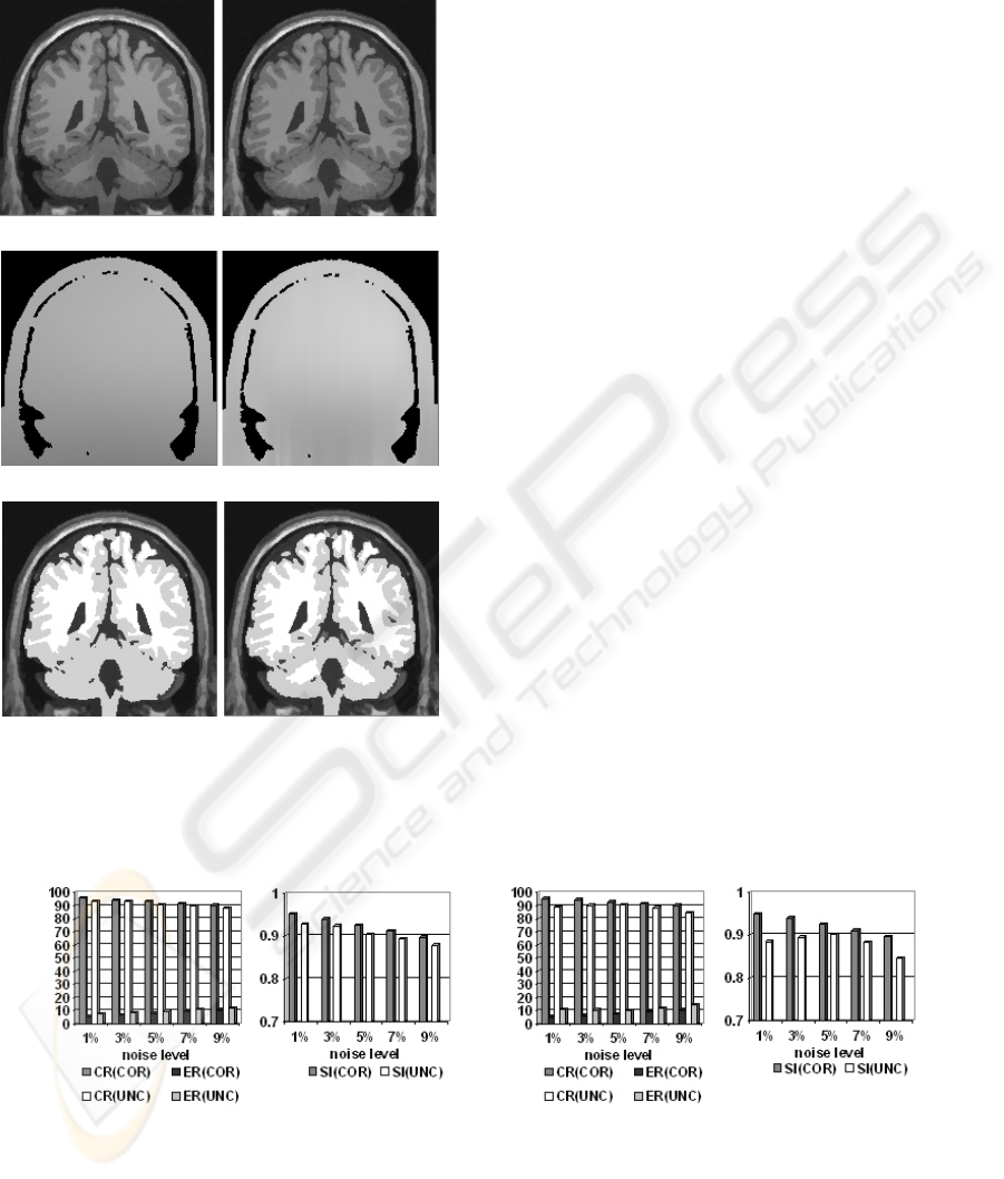
(a) uncorrected (b) corrected
(c) real bias field (d) estimated bias field
(e) uncorrected segmentation (f) corrected segmentation
Figure 5: Comparison of the results of uncorrected and
corrected simulated images (noise level=3%, RF=40%,
filtered).
The evaluations of the uncorrected (UNC) and
corrected (COR) simulated images with RF=20%
and with RF=40% are shown in Figure 6, where CR,
ER and SI are the average of GM and WM
respectively. They show that the bias correction
improved the performance of segmentation. After
bias correction the intensity inhomogeneities in the
images are compensated effectively both in RF=20%
and RF=40%. In addition, the results of our method
are compared with those from a popular brain
analysis technique called Statistical Parametric
Mapping (SPM) (Ashburner 2000). The software
package SPM2 was released in 2003
(http://www.fil.ion.ucl.ac.uk /spm/) and a procedure
for bias correction has been included. The
comparison (see Figure 7) indicates that our method
is comparable with SPM2. SPM2 uses an anatomical
atlas. Our method does not depend on such an atlas
and overcomes SPM2 for the noise levels 1%, 7%
and 9%. For the noise levels 3% and 5% SPM2
shows only slightly better results.
Unfortunately for real images the ‘ground truth’
is not available, so the same quantitative
measurement can not be conducted on them.
Therefore we only visually evaluated them. The
results with bias correction and without bias
correction are compared. There are no big
differences between them except for detailed
structures which can be detected by using bias
correction. In this paper we provide a segmentation
example of a real image with and without bias
correction (see Figure 8). The result with bias
correction seems to be appreciably better on some
detailed structures which are sketched out by circles.
Its 3D visualization result is also shown in Figure 8.
(a) RF=20% (b) RF=40%
Figure 6: Quantitive evaluation for the segmentation results of uncorrected and corrected simulated images.
IMPROVED SEGMENTATION OF MR BRAIN IMAGES INCLUDING BIAS FIELD CORRECTION BASED ON
3D-CSC
343
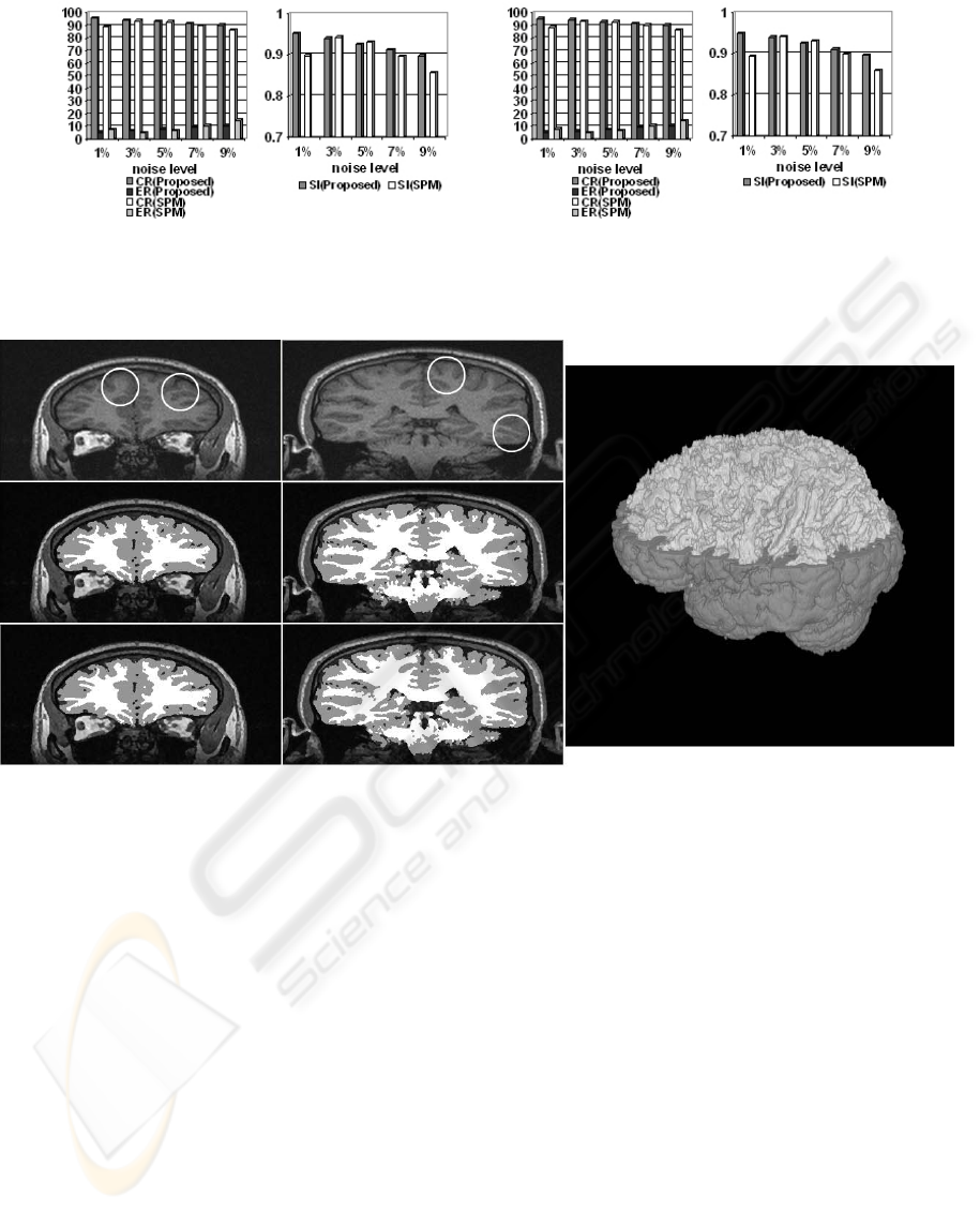
(a) RF=20% (b) RF=40%
Figure 7: Quantitative evaluation for the segmentation results of simulated images comparing the proposed method with
SPM2.
Figure 8: Comparison of the segmentation results of a real image with bias correction and without bias correction and its 3D
visualization. The original slices are in the first row. The segmentation results without bias correction are shown in the
second row. The third row shows the results with bias correction. Its 3D visualization is in the right column where the gray
matter is partially removed.
5 CONCLUSION
A fully automated, improved segmentation based on
the 3D-CSC for MR brain images is proposed in this
paper. In contrast to most existing methods, it is fast
with a satisfactory accuracy. It takes advantage of
the region- and intensity-based 3D-CSC and
combines it with further information from intensity
histograms to robustly segment MR brain images. A
bias correction is integrated into the method to
improve its performance. However, the results for
some images still indicate some problems: On the
one hand some detailed structures of the brain are
lost especially in the cerebellum, on the other hand
we sometimes are not able to remove all non-brain
tissues, i.e. sometimes small parts of non-brain
tissue around the eyes is still included. Those
problems depend on the size of the structuring
element of the morphological operations. A big
structuring element can avoid including more non-
brain tissues but some detailed structures of brain
may be lost and vice versa.
In the future we have to cope with the above
problems and want to segment and recognize other
significant structures in 3D MR brain images.
Furthermore, we want to compare our method with
other state of art brain segmentation techniques, i.e.
the Hidden Markov Random Field (HMRF)-based
method (Zhang 2001), and the fuzzy C-means
clustering (FCM)-based adaptive method (Liew
2003).
VISAPP 2006 - IMAGE ANALYSIS
344

REFERENCES
Ashburner, J., Friston, K. J., 2000. Voxel-based
morphometry-the methods. NeuroImage. 11(6Pt1):
805-821.
Carlotto, M. J., 1987. Histogram analysis using a scale-
space approach, IEEE Trans on PAMI. 9(1): 121-129.
Duda. R. O., Hart, P. E., Stork, D. G., 2001. Pattern
Classificatio, Wiley&SONS Press. London. 2
nd
edition.
Kuwahara, M., Hachimura, K., Eiho, S., 1976. Processing
of Ri-angiocardiographic images. Digital Processing
of Biomedical Images. Plenum Press. New York.
Liew, A. W., Yan, H., 2003. An adaptive spatial fuzzy
clustering algorithm for 3-D MR image segmentation.
IEEE Trans on Medical Imaging. 22(9): 1063-1075.
MacDonald, D., Kabani, N., Avis, D., 2000. Automated 3-
D extraction of inner and outer surfaces of cerebral
cortex from MRI. Neuroimage. 12(3): 340-356.
Pham, D. L., Xu, C. Y., Prince, J. L., 2000. Current
methods in medical image segmentation, Annual
Review of Biomedical Engineering. 2: 315-337.
Priese, L., Sturm, P., Wang, H. J., 2005. Hierarchical Cell
Structures for Segmentation of Voxel Images. In
SCIA2005, 14
th
Scandinavian Conference on Image
Analysis. Springer Press.
Rajapakse, J. C., Kruggel, F., 1998. Segmentation of MR
images with intensity inhomogeneities. Image Vision
Computing. 16(3): 165-180.
Rehrmann, V., Priese, L., 1998. Fast and robust
segmentation of natural color scenes. In ACCV98. 3
rd
Asian Conference on Computer Vision. Springer Press.
Schnack, H. G., Hulshoff Pol, H. E., Baare, W. F., 2001.
Automated separation of gray and white matter from
MR images of the human brain, Neuroimage. 13(1):
230-237.
Sled, J. G., Zijdenbos, A. P., Evans, A. C., 1998. A
nonparametric method for automatic correction of
intensity nonuniformity in MRI data. IEEE Trans on
Medical Imaging. 17(1): 87-97.
Stokking, R., Vincken, K. L., Viergever, M. A., 2000.
Automatic morphology-based brain segmentation
(MBRASE) from MRI-T1 Data. NeuroImage. 12(6):
726-738.
Sturm, P., 2004. 3D-Color-Structure-Code. A new non-
plainness island hierarchy. In ICCSA 2004,
International Conference on Computational Science
and Its Applications. Springer Press.
Suzuk, H., Toriwak, J., 1991. Automatic segmentation of
head mri images by knowledge guided thresholding.
Computerized Medical Imaging and Graphics. 15(4):
233-240.
Vovk, U., Pernus, F., Likar, B., 2004. MRI intensity
inhomogeneity correction by combining intensity and
spatial information, Physics in Medicine and Biology.
49: 4119-4133.
Wells III, W. M., Grimson, W. E. L., Kikinis, R. Jolesz, F.
A. 1996. Adaptive segmentation of MRI data. IEEE
Trans on Medical Imaging. 15(4): 429-442.
Zhang, Y. Y., Brady, M., Smith, S., 2001. Segmentation
of brain MR images through a hidden markov random
field model and the expectation-maximization
algorithm. IEEE Trans on Medical Imaging. 20(1): 45-
57.
IMPROVED SEGMENTATION OF MR BRAIN IMAGES INCLUDING BIAS FIELD CORRECTION BASED ON
3D-CSC
345
