
CONVOLUTION KERNEL COMPENSATION APPLIED TO 1D
AND 2D BLIND SOURCE SEPARATION
Damjan Zazula, Aleš Holobar, Matjaž Divjak
Faculty of Electrical Engineering and Computer Science, University of Maribor
Smetanova 17, 2000 Maribor, Slovenia
Keywords: Blind source separation, Convolution kernel compensation, Bioelectrical signal decomposition,
Range imaging.
Abstract: Many practical situations can be modelled with multiple-input multiple-output (MIMO) models. If the input
sources are mutually orthogonal, several blind source separation methods can be used to reconstruct the
sources and model transfer channels. In this paper, we derive a new approach of this kind, which is based on
the compensation of the model convolution kernel. It detects the triggering instants of individual sources,
and tolerates their non-orthogonalities and high amount of additive noise, which qualifies the method in
several signal and image analysis applications where other approaches fail.. We explain how to implement
the convolution kernel compensation (CKC) method both in 1D and 2D cases. This unified approach made
us able to demonstrate its performance in two different experiments. A 1D application was introduced to the
decomposition of surface electromyograms (SEMG). Nine healthy males participated in the tests with 5%
and 10% maximum voluntary isometric contractions (MVC) of biceps brachii muscle. We identified 3.4 ±
1.3 (mean ± standard deviation) and 6.2 ± 2.2 motor units (MUs) at 5% and 10% MVC, respectively. At the
same time, we applied the 2D version of CKC to range imaging. Dealing with the Middlebury Stereo Vision
referential set of images, our method found correct matches of 91.3± 12.1% of all pixels, while the obtained
RMS disparity difference was 3.4 ± 2.5 pixels. This results are comparable to other ranging approaches, but
our solution exhibits better robustness and reliability.
1 INTRODUCTION
Blind source separation (BSS) has matured to a very
well established theory which has given a fresh im-
petus to several applications in different research
fields. If a problem can be modelled in multiple-
input multiple-output sense (MIMO) and the input
excitations of such a model can be considered or-
thogonal sources, many BSS techniques are available
to separate those sources. Robust and useful solu-
tions have been reported for telecommunications
(Madhow, 1998), seismic and radar signals (Desodt,
1994), speech processing (Gribonval, 2002), bioelec-
tric signals (Barros, 1999), image processing (Hy-
värinen, 2002), etc.
The majority of BSS-based approaches take ad-
vantage of the sources’ orthogonality. Several obser-
vations, i.e. the output signals of the presumed
MIMO model, are taken into account referring to
their mutual information contents, such as covariance.
The covariance-based techniques build a covariance
matrix which comprises the information on the model
transfer channels, i.e. the model convolution kernel,
and the covariance of sources. Actually, the source
covariance matrix appears to be diagonal, which un-
veils the convolution kernel. The information on the
convolution kernel is, afterwards, used to deconvolve
also the original source signals (Cardoso, 1998), (Be-
louchrani, 1997).
However, there are two major drawbacks that
degrade the success of BSS in certain cases, which is
when the number of observations is lower than the
number of sources and when the sources lack the
orthogonality. The both drawbacks prevent a proper
identification of the convolution kernel, which hin-
ders applications in the biomedical field, for example.
The obtained shapes of source signals and modelled
channel responses are distorted because they are pro-
jected into an orthogonal space, in underdetermined
cases also with lower number of dimensions as
126
Zazula D., Holobar A. and Divjak M. (2006).
CONVOLUTION KERNEL COMPENSATION APPLIED TO 1D AND 2D BLIND SOURCE SEPARATION.
In Proceedings of the International Conference on Signal Processing and Multimedia Applications, pages 126-133
DOI: 10.5220/0001568801260133
Copyright
c
SciTePress

needed. So, the obtained results equal unknown linear
combinations of the original sources and channel
responses.
Recently, a novel approach was proposed which
successfully separates the contributions of sources
even if they are only close-to-orthogonal and if the
number of observations is underdetermined (Holobar,
2004). It is based on the fact that there is variety of
situations where sources produce only a limited num-
ber of finite symbols (source activity). Being sent
through the transfer channel, those symbols are con-
volved with the channel responses and they appear in
the observations as the contributions of symbols. If,
for example, bioelectric signals are considered, elec-
trocardiograms (ECG) can be modelled with fully
orthogonal sources (there is no overlap possible be-
tween different types of heart beats, such as normal
systoles and extrasystoles), while electromyograms
(EMG) lose orthogonality with increasing contraction
forces (motor-unit action potentials exhibit more
overlapping) (De Luca, 1996). On the other hand,
observing certain types of communications, such as
CDMA (Madhow, 1998), orthogonality of sources
may be supposed as well. Moreover, we are not con-
strained to 1D; similar reasoning may be extended to
2D images. If an image is taken as a MIMO output
observation, it can also be considered the result of
some source activities transferred through the model
channels. In this case, sources produce symbols in the
form of 2D regions (subimages that contribute to the
observed image), and are expected to be orthogonal
(subimages do not overlap).
Given a number of observations of some sources,
the contributions produced by the transferred source
symbols may be characterized by their shape and
appearance (triggering) instants. Stationarity is also
supposed both for the sources and for the model
channels. We have developed a method which makes
use of the abovementioned facts and detects the trig-
gering instants of the same symbols as they appear in
the observation. Our method actually compensates
the detected shape of the observed source contribu-
tions. The approach turned out to be Bayesian opti-
mal (Kay, 1993).
The paper continues as follows: Section 2 reveals
the novel method called convolution kernel compen-
sation (CKC) and extends it from 1D to 2D, Section 3
explains its application to surface EMG signals, while
section 4 shows the method’s efficiency when applied
to range imaging in stereo vision. The paper is con-
cluded by Section 5.
2 DETECTION OF SOURCE-
SYMBOL TRIGGERING
INSTANTS
Consider the following data model:
∑∑
=
−
=
=+−=
K
j
L
l
ijiji
Minvlntlcny
1
1
0
,,1);()()()( … (1)
where y
i
(n) stands for the i-th observation, c
ij
(l) cor-
responds to the contribution of length L of the j-th
source symbol in the i-th observation, and t
j
(n-l)
denotes a sequence of triggering instants for this
symbol,
∑
∞
−∞=
−=
l
jj
lTnnt ))(()(
δ
, with unit-sample
pulses placed at T
j
(l) lags, while v
i
(n) is considered
i.i.d. white noise independent from the sources.
It has been shown 0 that Eq. (1) can be trans-
formed into a multiplicative vector form as follows:
1,,0);()()( −=
+
=
Nnnnn
eeee
…vtCy (2)
where subscript e designates extended vectors and
matrices, C
e
contains the observed contributions of
source symbols,:
⎥
⎥
⎥
⎦
⎤
⎢
⎢
⎢
⎣
⎡
=
MKM
K
e
CC
CC
C
1
111
(3)
with
⎥
⎥
⎥
⎦
⎤
⎢
⎢
⎢
⎣
⎡
−
−
=
)1()0(0
0)1()0(
Lcc
Lcc
ijij
ijij
ij
C
, (4)
y
e
(n) stands for the extended vector of observations,
and t
e
(n) for the vector of triggering pulses, both at
lag n:
T
eK
Kee
T
eM
Mee
MLnt
ntMLntntn
Mny
nyMnynyn
)]2(
),....,(),....,2(),....,([)(
)]1(
),....,(),....,1(),....,([)(
11
11
+−−
+−−=
+−
+−=
t
y
(5)
Extended noise vector v
e
(n) is considered constructed
in the same way.
M
e
from Eqs. (5) means an extension factor. If it
fulfils the following inequality
)1(
−
+
≥
⋅
ee
MLKMM ,
(6)
then for K different observed symbols of length L and
M observations the matrix C
e
is of full column rank.
This condition warranties a successful elimination of
contributions of C
e
, as we are going to show in the
next subsection.
CONVOLUTION KERNEL COMPENSATION APPLIED TO 1D AND 2D BLIND SOURCE SEPARATION
127

2.1 Convolution Kernel
Compensation
Recall Eq. (2). It has a typical MIMO structure. From
this point of view, C
e
is a convolution kernel convolv-
ing t
e
(n) to observations y
e
(n). Given y
e
, if we can get
rid of C
e
the triggering instants of unknown source
symbols, t
e
, would result. We called this process
“convolution kernel compensation (CKC)”.
Observe the following expression:
)()(
1
nn
e
T
e
e
yRy
y
−
(7)
where
e
y
R
stands for the sample correlation matrix:
ICRCICttCyyR
ty
22
σσ
+=+==
T
ee
T
e
T
eee
T
ee
ee
(8)
with
e
t
R
denoting sample correlation matrix of
source triggering trains of pulses, and the expression
σ
2
I stands for the correlation matrix of noise v
e
.
For easier comprehension of derivation, continue
with the noise-free case. By substituting (8) into (7),
we see that convolution kernel is eliminated:
)()(
)()()()(
1
111
nn
nnnn
e
T
e
eee
T
e
T
e
T
ee
T
e
e
ee
tRt
tCCRCCtyRy
t
ty
−
−−−−
==
(9)
The expression from (7) is known as Mahalanobius
distance, which, as it is clear from Eq. (9), yields only
the information on source triggering instants. Actu-
ally, its value depends on the number of sources ac-
tive in given time instant n. This is why we call it
activity index.
Suppose we deal with orthogonal sources and n
0
indicates the time instant where one of them gener-
ates a symbol (its contribution appears in the observa-
tion). Then vector t
e
(n
0
) is all zero except the element
which belongs to the generated symbol, say the i-th,
and equals 1. Besides, matrix
e
t
R
is diagonal, and so
is
1−
e
t
R
. It is then straightforward that
)()()(
)()()()()(
,,,0,,
1
0
1
0,
0
ntrntntr
nnnnnp
ieiiieieii
e
T
ee
T
ein
ee
=
===
−−
tRtyRy
ty
(10)
where r
i,I
denotes the i-th diagonal element of
1−
e
t
R ,
and t
e,i
(n) stands for the train value at lag n for the i-th
source symbol. Evidently, in Eq. (10) we have ob-
tained a sequence
in ,
0
p
whose values equal the i-th
source-symbol triggering pulse train to a constant
amplitude factor, r
i,i
. So, all repetitions of that symbol
are detected.
The values of activity index indicate those lags n
i
where individual sources contribute their symbols. If
we select such n
i
’s that cover all different source con-
tributions, a thorough decomposition is done and all
source-symbol triggering pulse trains,
t
i
; i∈[1,K], are
separated.
Let’s also briefly discuss nonideal conditions. In
ideal condition with orthogonal source-symbol con-
tributions, no noise and the number of observations
exceeding the number of different source-symbol
contributions, the convolution kernel
C
e
is completely
eliminated. If any of the ideal conditions cannot be
met,
C
e
is not eliminated but only compensated to a
certain extent. Consequently, the resulting decompo-
sition of source-symbol triggering instants, Eq. (10),
move off the ideal binary valued pulse train (sample
values either 0 or r
i,i
). Hence, the ideal Bernoulli dis-
tribution of any
jn
i
,
p
tends to “smear”, so the prob-
ability distribution of “no trigger” values may start
overlapping the distribution of “trigger” values. A
more detailed explanation goes beyond the scope of
this paper, so we only stress here that even in far non-
ideal cases, such as with the signal-to-noise ratio as
low as 0 dB, confidence level for the detection of
source-symbol triggering instants remain above 98 %.
Some additional results are given in the experimental
part, Sections 3 and 4.
2.2 Extension to 2D Cases
As we have pointed out, analogy between source con-
tributions in 1D and 2D observations can be found.
2D observations, i.e. images, can be interpreted as a
compositum of several subimages appearing at differ-
ent image co-ordinates. Thus, an image may be seen
as a convolution of different regions and the corre-
sponding “triggering” unit-samples whose positions
in 2D determine the region placements within the
image frame.
The most obvious way to implement CKC also
in 2D is vectorization of images. Assume we have set
of images
I
k
; k∈[1,M], and that I
k
(i,j) denotes the
value of the k-th image pixel at (i,j) co-ordinates.
Then
y
k
=vec(I
k
) (11)
is a vector whose elements correspond to the con-
catenated rows of image
I
k
, so that
)]1,1(
,),1,1(),0,1(
,,),1,1(,),1,1(),0,1(
,),1,0(,),1,0(),0,0([)(
21
11
2
2
−−
−−
−
−=
NNI
NINI
NIII
NIIIvec
k
kk
kkk
kkkk
…
……
…
0
0I
(12)
SIGMAP 2006 - INTERNATIONAL CONFERENCE ON SIGNAL PROCESSING AND MULTIMEDIA
APPLICATIONS
128

where N
1
and N
2
stand for image dimensions. Every
row of pixels is padded by M
e
zeros (denoted by vec-
tor
0), where M
e
means the extension factor from
inequality (6).
The extension of vector
y
k
from Eq. (11) is per-
formed the same way as for 1D case in Eq. (5). Also
the other decomposition steps explained in Eqs. (7) to
(10) can be implemented without modifications. A
selected n
0
now determines location of a certain
subimage region, with its 2D co-ordinates being
transformed into n
0
by vectorization. The resulting
sequence
in ,
0
p
comprises pulses at the positions indi-
cating the repetitions of the subimage from location
n
0
. For optimal decomposition results, the number of
observations, M, meaning different images of the
same scene here, must exceed the number of different
subimages.
It has to be emphasized that in Eq. (12) proposed
image vectorization leads to a one-row vector, which
limits the decomposition to subimages of one-row
width only. At the same time, these subimages can
extend at most across M
e
image columns, because the
CKC extension introduced in Eq. (5) “joins” the in-
formation of M
e
subsequent samples. If the subimage
regions of interest span larger areas, images have to
be vectorized differently. They have to be segmented
in such a way that the number of rows in every seg-
ment corresponds to the vertical dimension of the
regions looked for. Every segment row is then taken
as a separate observation entering the CKC-based
decomposition. Consequently, only a single image
segment is decomposed at a time, with no correlation
to other segments. However, it is also possible for
several image segments to be included into the same
decomposition run. In this case, those segments have
to be padded by M
e
zeros and concatenated.
3 APPLICATION OF CKC TO
THE SURFACE
ELECTROMIOGRAM
DECOMPOSITION
Human body contains different kinds of electrically
excitable tissues, such as nerves and muscle fibres,
which, when active, conduct measurable biopoten-
tials, typically of length of several ms. These biop-
tentials can be detected either by inserting invasive
needle electrodes into the tissue or by placing pick-
up electrodes on the skin surface, above the investi-
gated organ. Although being more selective, the in-
vasive needle electrodes impose several restrictions
to everyday clinical investigations. Firstly, measure-
ments must be taken in a sterile environment and
under supervision of trained physicians. Secondly, in
order to reduce the tissue damage, there is a constant
need for miniaturization of needle electrodes. This
significantly increases the costs of manufacturing.
Finally, the invasive recoding techniques put a lot of
stress on an investigated subject and increase the fear
from preventive clinical investigations (Merletti,
1994).
The aforementioned problems can be avoided by
using less selective surface electrodes, providing
signal processing techniques exists, which are capa-
ble of extracting clinically relevant information out
of recorded data. Unfortunately, this is not a trivial
task. Namely, the supportive tissues separating the
investigated biological sources from the pick-up
electrodes acts as a low pass filter and hinder the
information in the detected signals. In addition, ac-
quiring surface signals, contributions of different
biological sources are detected. When electrical ac-
tivity of skeletal muscles is observed, for example,
we deal with several tens of sources (so called motor
units, MU), simultaneously contributing their biopo-
tentials (so called action potentials, AP) to the de-
tected EMG interference pattern (Merletti, 1994).
The decomposition of the surface EMG into the con-
tributions of different MUs is, hence, a highly com-
plex problem whose solution has been addressed
with a many different methods. Unfortunately, most
methods suffer from a drop of performance in case of
significant superposition of MU action potentials.
Surface EMG signals can always be modeled
by Eq. (1), provided they have been acquired during
an isometric muscle contraction (De Luca, 1996). In
such a model, observations y
i
(n) correspond to
measured surface signals, c
ij
(n) corresponds to the
action potential of the j-th MU, as detected by the i-
th pick-up electrode, while t
j
(n) stands for a pulse
sequence carrying the information about triggering
times of APs. The length of detected APs, L, de-
pends on the sampling frequency, but typically
ranges from 15 to 25 samples when the Nyquist
frequency is made equal to the bandwidth of the
surface signals. At low contraction levels, different
MUs discharge in relatively regular but random time
instants, independently of each other. At higher con-
traction levels, the MUs start exhibiting weak ten-
dency to synchronize, but this synchronization
hardly exceeds the 5 % of its maximal possible
value. As a result, t
j
(n) can be modelled as close-to-
orthogonal random pulse sequences and the theory
of 1D CKC method can be readily applied to the
SEMG signals. This is further demonstrated by the
CONVOLUTION KERNEL COMPENSATION APPLIED TO 1D AND 2D BLIND SOURCE SEPARATION
129
experimental results described in the next subsec-
tion.
3.1 Experimental Protocol
Nine healthy male subjects (age 26.8 ± 2.2 years,
height 179 ± 7 cm, weight of 72.1 ± 8.3 kg) partici-
pated to our experiment. Surface EMG signals were
acquired during isometric, constant-force contractions
of the dominant biceps brachii muscle. In order to
provide sufficient number of measurements, M, a
matrix of 55 pick-up electrodes arranged in five col-
umns and 11 lines (without the four corner electrodes)
was used while all the contractions were performed at
5% and 10% of the maximum voluntary contraction
(MVC) force. The EMG signals were recorded in
longitudinal single differential configuration, ampli-
fied (gain set to 5000), band-pass filtered (3 dB
bandwidth, 10 –500 Hz), and sampled at 2500 Hz by
a 12 bit A/D converter. During signal acquisition, the
noise and movement artefacts were visually con-
trolled and reduced by applying water to the skin sur-
face. Before any further processing, all the measure-
ments were digitally filtered to suppress the power-
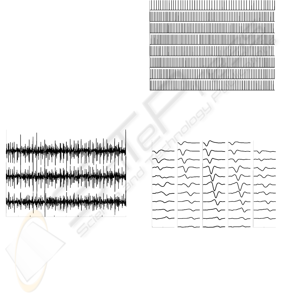
line interference. Recorded signals are exemplified in
Fig. 1.
0.2 0.4 0.6 0.8 1 1.2 1.4 1.6 1.8 2
1
2
3
Time [s]
Measurements
0.2 0.4 0.6 0.8 1 1.2 1.4 1.6 1.8 2
1
2
3
Time [s]
Measurements
Figure 1: Real surface EMG signals recorded during isomet-
ric, low-level (10% MVC) contraction of dominant biceps
brachii muscle.
The measured signals were extended according to
Eq. (5) with extension factor, M
e
, set to 10. In order to
reconstruct the MU triggering pulses (Fig. 2), 1D
CKC decomposition method was applied to the
measured signals. The identified triggering pulses
were then used by spike triggering sliding window
averaging technique (Disselhorst-Klug, 1999) to re-
construct the MU APs as detected by different pick-
up electrodes (Fig. 3 depicts the first decomposed AP
as it contributes to each of 51 electrodes). Finally,
convolving the estimated AP shapes with the identi-
fied sequence of MU triggering pulses, the MU AP
trains were reconstructed and compared to the origi-
nal measurements (Figs. 4.a and 4.b). Rows 1 to 10 in
Fig. 4 correspond to the ten decomposed MU APs
depicted in the time instants when they trigger and
contribute to the measured SEMGs. They are
summed up in row 4.b).
23.6 24.4 25.2 26 26.8 27.6 28.4 29.2 30
1
2
3
4
5
6
7
8
Time [s]
MU
23.6 24.4 25.2 26 26.8 27.6 28.4 29.2 30
1
2
3
4
5
6
7
8
Time [s]
MU
Figure 2: A part of MU triggering pulses (i.e. time instants
in which the contributions of different MUs appeared in
observations) reconstructed by the 1D CKC method from 30
s long real SEMG signals of dominant biceps brachii muscle
(subject 3, 10% MVC measurement).
2 3
Columns of electrodes
41
11
10
9
8
7
6
5
4
3
2
1
Rows of electrodes
52 3
Columns of electrodes
41
11
10
9
8
7
6
5
4
3
2
1
Rows of electrodes
5
Figure 3: APs of MU 1 reconstructed by the spike triggered
sliding window averaging technique (293 averages accord-
ing to the train depicted in Fig. 2, bottom) from given 30 s
long SEMG observations.
On average, 3.4 ± 1.3 (mean ± standard deviation)
and 6.2 ± 2.2 MUs were identified during the contrac-
tions at 5% and 10% MVC, respectively. The exact
number of active MUs is, of course, unknown. Never-
theless, comparing the energies of the identified MU
action potentials with the energy of the original signal
we can approximately estimate the percentage of the
information that was extracted from the surface EMG
SIGMAP 2006 - INTERNATIONAL CONFERENCE ON SIGNAL PROCESSING AND MULTIMEDIA
APPLICATIONS
130
signals. The average ratio yielded 71 ± 15%, proving
that the largest SEMG components were identified
(Fig. 4). Most of the identified MUs showed decreas-
ing firing frequency over time (presumably due to
fatigue).
19.05 19.1 19.15 19.2 19.25 19.3 19.35 19.4
1
2
3
4
5
6
7
8
9
10
b)
a)
Time [s]
Motor units
19.05 19.1 19.15 19.2 19.25 19.3 19.35 19.4
1
2
3
4
5
6
7
8
9
10
b)
a)
Time [s]
Motor units
Figure 4: Contributions of different MUs identified by the
1D CKC method from 30 s long real SEMG signals re-
corded during isometric, 10% MVC measurement of the
dominant biceps brachii (subject 8); a) the originally ob-
served SEMG signal, b) sum of the identified MU contribu-
tions.
Finally, the shapes of the MU action potentials as
detected by the different electrodes were stable over
time and indicated anatomical and physiological MU
properties, such as location of innervation zones,
length of the fibres, and muscle fibre conduction ve-
locity (Fig. 3).
4 APPLICATION OF CKC TO
RANGE IMAGING
Human beings depend on stereo vision for observing
their surroundings. Slight displacement of images
enables them to reliably detect range information,
which can be used to their advantage. In computer
vision, the same effect is used to reconstruct the
range or depth image of a scene based on two or
more input images. Range reconstruction can be
formulated as a matching problem between pixels of
the left and right stereo image. In general, the prob-
lem doesn't have a unique solution due to lack of
image texture, occlusions, periodic image structures
and noise (Šara, 2002). Early algorithms avoided
those problems by reconstructing only sparse range
images (Sonka, 1994). Modern applications, such as
image-based modelling, texture mapping of 3D ob-
jects and similar, require dense range images, where
disparity of almost all image pixels is known. To
alleviate this problem, several constraints are com-
monly used. All the surfaces in the scene are sup-
posed to be Lambertian, the geometry of the stereo-
system should be known (calibrated camera) and
range values are expected to change smoothly, with-
out sharp jumps (Gutierrez, 2003).
Using the geometric properties of the stereosys-
tem, it can be shown that the matching space can be
reduced to two epipolar image rows (Jain, 1995).
Each image row can easily be represented as an ob-
servation
y
k
, extended and decomposed by the CKC
method, referring to the extension introduced in Sub-
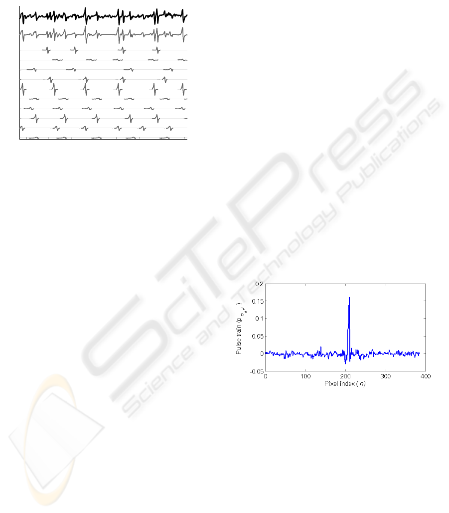
section 2.2. In order to detect disparity of every
pixel, its position in the left image row is described
by index n
0
and the pulse train
in ,
0
p
is calculated
according to Eq. (10) along the right epipolar image
row. Ideally, the sequence
in ,
0
p
contains only one
sharp impulse. This pulse indicate the most probable
location n
1
of the subimage which best corresponds
in the right stereo image to that selected by index n
0
in the left image (Fig. 5). Disparity of pixel n
0
is,
therefore, calculated as
Disp(n
0
) = n
0
– n
1
. (13)
In order to achieve more reliable and robust re-
sults, the matching is repeated using the right stereo
image as a starting point. Only pixels with consistent
left-to-right and right-to-left matches are assigned the
final disparity value.
Figure 5: An example of a pulse train
in ,
0
p
, as obtained for
a selected row in the right image. The location of the pulse
determines the location of a suitable subimage region.
As we have explained in Subsection 2.2, the
shape of image regions being matched by our CKC
approach is determined by the number of image rows
included in one decomposition run, and by the exten-
sion factor M
e
. The quality of left-right stereo-image
matching depends on the appearance of the same im-
age regions in both left and right images. This ap-
pearance may not be equally good for smaller or lar-
ger sections of an image object. So, it can be expected
that its depth may be misinterpreted owing to inferior
quality of matching. However, if we observe a part of
CONVOLUTION KERNEL COMPENSATION APPLIED TO 1D AND 2D BLIND SOURCE SEPARATION
131

an object in different sizes, so with different size of
regions inserted in the CKC-based matching, the in-
formation of best fit can be compared for different
region sizes. Thus, the most probable disparity can be
estimated, which is the idea followed by our 2D CKC
range imaging, as exemplified in the next subsection.
4.1 Experiments with CKC-based
range imaging
All experiments were performed on the test images
from the Middlebury Stereo Vision Page (Scharstein,
2002). This test set provides reliable reference data
and is very popular in the research community, ena-
bling the comparison of different range reconstruction
techniques. The results of our CKC-based approach
are depicted in Fig. 6.
a)
b)
c)
Figure 6: An example of reconstructed range image on the
SAWTOOTH stereo test set: (a) left input image, (b) refer-
ence range image, and (c) the resulting CKC-based range
image.
In Table 1, they are compared to results of the
standard correlation-based approach using the follow-
ing performance metrics:
o percentage of image pixels with consistent
left-to-right and right-to-left matches,
o percentage of matched pixels whose disparity
differs from the reference value by more than
1 pixel,
o RMS of disparity difference between matched
pixels and the reference image.
Table 1: Comparison of disparity values, obtained the 2D
CKC method and a typical correlation-based approach
(SSD, 5×5 window). Mean values for four test images
(MAP, TSUKUBA, VENUS, SAWTOOTH) are shown.
Algorithm
Matches
found
(%)
Bad
matches
(%)
RMS dis-
parity
difference
(pixels)
CKC
91.3 ±
12.1
1.6 ± 0.4 3.4 ± 2.5
SSD
78.2 ±
14.2
2.0 ± 0.5 7.9 ± 4.5
5 CONCLUSIONS
We derived a novel method for statistical signal
processing which blindly separates source
contributions superimposed in one or more available
observations. It is based on the correlation of
SIGMAP 2006 - INTERNATIONAL CONFERENCE ON SIGNAL PROCESSING AND MULTIMEDIA
APPLICATIONS
132

observations, so that the inverse of correlation matrix
is used to compensate the convolution kernel
influence. The method tolerates moderate declines of
sources from the orthogonality, and copes with
considerable amount of additive random noise.
1D version of our CKC approach was applied to
the decomposition of real surface EMG signals. The
reported results demonstrate the CKC method is not
sensitive to superimpositions of MU action potentials
and has high potential in clinical applications for the
non-invasive analysis of single MU properties.
In this paper we also derived a 2D version of
CKC. It makes use of all the benefits mentioned
above also for image processing. One of possible
applications is searching equivalent regions in more
images, whereas the matching on a pair of stereo im-
ages directly imposes a new range imaging technique.
We exemplified it by constructing range images for a
set of reference images. The obtained results are
comparable with other known approaches, but be-
cause of the CKC being rather noise resistant, the
new way of range imaging obtains a better robust-
ness.
Recent investigations prove that the CKC per-
formance can be improved by combining it with non-
linear modifications of observations and by non-
linear modelling instead of present MIMO scheme.
Our research continues in this direction.
REFERENCES
Madhow, U., 1998. Blind Adaptive interference suppression
for direct-sequence CDMA. In Proceedings of the
IEEE, 86 (10), 2049-2069.
Desodt G.., Muller D., 1994. Complex independent compo-
nents analysis applied to the separation of radar signals.
In Signal Processing V, Theories and applications, 665-
668.
Gribonval R., 2002. Sparse decomposition of stereo signals
with matching pursuit and application to blind separa-
tion of more than two sources from a stereo mixture. In
Proceedings of ICASSP’02.
Barros A. K., Mansour A., Ohnishi N., 1999. Removing
artefacts from ECG signals using independent compo-
nents analysis. In Neurocomputing, 22, 173-186.
Hyvärinen A., Inki M., 2002. Estimating overcomplete in-
dependent component bases for image windows. In
Journal of Mathematical Imaging and Vision, 17, 139-
152.
Cardoso J. F., 1998. Blind signal separation: statistical prin-
ciples. In Proceeding of the IEEE, Special issue on
blind identification and estimation, 9 (10), 2009-2025.
Belouchrani A., Meraim K. A., Cardoso J. F., Moulines E.,
1997. A blind source separation technique based on
second order statistics. In IEEE Transactions on signal
processing, 45 (2), 434-444.
Holobar A., Zazula D., 2004. Correlation-based approach to
separation of surface electromyograms at low contrac-
tion forces. In Med. & Biol. Eng. & Comput., 42 (4),
487-496.
Merletti R., 1994. Surface electromyography: possibilities
and limitations. In J. of Rehab. Sci., 7 (3), 25-34.
De Luca C. J., Foley P. J., Erim Z., 1996. Motor unit control
properties in constant-force isometric contrac-tions. In
J. of Neurophysiol., 76 (3), 1503-1516.
Disselhorst-Klug C., Rau G.., Schmeer A., Silny J., 1999.
Non-invasive detection of the single motor unit action
potential by averaging the spatial potential distribution
triggered on a spatially filtered motor unit action poten-
tial. In J. of Electromyogr. and Kinesiol, 9, 67-72.
Kay S. M., 1993. Fundamentals of Statistical Signal Proc-
essing, Prentice-Hall International. London.
Šara R., 2002. Finding the largest Unambiguous Component
of Stereo Matching. In European Conference on Com-
puter Vision, LNCS 2352, 900-914.
Sonka M., Hlavac V., Boyle R., 1994. Image Processing,
Analysis and Machine Vision, Chapman & Hall. Lon-
don.
Gutierrez S., Marroquin J. M., 2003. Disparity estimation
and reconstruction in stereo vision. In Technical report,
Centro de Investigacion en Matematicas, Mexico.
Jain R., Kasturi R., Schunck B. G., 1995. Machine Vision,
McGraw-Hill Inc. International Edition.
Scharstein D., Szeliski R., 2002. A Taxonomy and Evalua-
tion of Dense Two-Frame Stereo Correspondence Algo-
rithms. In International Journal of Computer Vision, 47,
7-42.
CONVOLUTION KERNEL COMPENSATION APPLIED TO 1D AND 2D BLIND SOURCE SEPARATION
133
