
PROCESSING OF NON-STATIONARY SIGNAL USING
LEVEL-CROSSING SAMPLING
Modris Greitans
Institute of Electronics and Computer Science
14 Dzerbenes str., Riga, LV1006, LATVIA
Keywords:
Clock-less design, non-stationary signal, level-crossing sampling, time-frequency representation.
Abstract:
The spectral characteristics of multimedia signals typically vary with time. Preferably, the sampling density of
them would comply with instantaneous bandwidth of signal. The paper discusses the level-crossing sampling
principle, which provides such capability for analog-to-digital conversion. As the captured samples are spaced
non-uniformly, the appropriate digital signal processing is required. The non-stationary signal is characterized
by time-frequency representation. Its classical approaches are inspected for applicability to analyze the data
obtained by level-crossing sampling. Several enhancements of short-time Fourier transform approach are
proposed, which are based on the idea to minimize the reconstruction error not only at sampling instants,
but also between them with the same accuracy. Additional benefits are gained if the instantaneous spectral
range of analysis is complied with local sampling density: artifacts are removed, complexity of calculations
is decreased. The performance of algorithms is demonstrated by simulations. Presented research can be
attractive for clock-less designs, which receive now an increasing interest. Their promising advantages can
play a significant role in future electronics’ development.
1 INTRODUCTION
Conventional digital signal processing techniques of-
ten consider the stationarity of a signal within a frame
of analysis. It is assumed that the statistical charac-
teristics of signal do not change with time. The con-
cept of stationarity provides the possibility of fixing
the sampling rate (it should be at least twice as high
as the maximum signal frequency), as well as of con-
structing effective processing methods, for example
the Discrete Fourier transform (DFT). However, nat-
ural signals typically are time-varying, and they can
be a mixture of events localized both in time and fre-
quency (Akay, 1998).
Intuitively speaking, the non-stationarity of a sig-
nal should be reflected in the process of analog-to-
digital (A/D) conversion. For example, let us inspect a
signal with high instantaneous frequency regions and
low instantaneous frequency in other regions. It is
more efficient to sample the low frequency regions at
a lower rate than the high frequency regions. Con-
sequently, with appropriate non-equidistantly spaced
samples one might approximate a signal with fewer
samples per interval than in the uniform sampling
case, where sampling frequency is defined taking into
account only the highest signal component. Two con-
clusions follow: non-uniform sampling is the natu-
ral choice for the discrete representation of a non-
stationary signal, and the non-uniformity of sampling
process has to be caused by the local properties of sig-
nal.
The work presented in this paper is based on the
idea of abandoning traditional clock-driven A/D con-
version and the uniform digital signal processing,
which typically follows it. Instead of that, a clock-
less structure of data processing system is suggested,
where the A/D conversion is signal-driven. To illus-
trate the difference, the processing chains of both ap-
proaches are illustrated in the Fig.1. Let us empha-
size the key benefits of the asynchronous electron-
ics: lower power consumption, absence of the clock
screw, reduced heat elimination, lower EMI, auto-
matic adaptation to physical properties, etc. (Hauck,
1995). The popular types of signal-dependent sam-
pling are based on zero-crossing, reference signal
crossing, level-crossing or send-on-delta concepts.
Each of them has its own advantages and limitations,
however joint features are: the signal samples can
be spaced non-uniformly, local sampling density de-
pends on local properties of signal, and it is impos-
170
Greitans M. (2006).
PROCESSING OF NON-STATIONARY SIGNAL USING LEVEL-CROSSING SAMPLING.
In Proceedings of the International Conference on Signal Processing and Multimedia Applications, pages 170-177
DOI: 10.5220/0001569001700177
Copyright
c
SciTePress
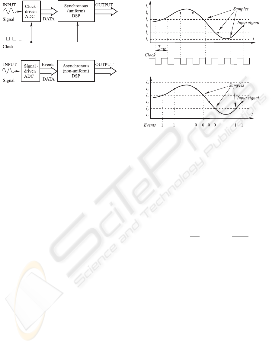
(a)
(b)
Figure 1: Structures of DSP system based on different
paradigm: synchronous (a), asynchronous (b).
sible to determine the sampling time instants in ad-
vance. The paper discusses digital signal processing
if the level-crossing sampling scheme is used to cap-
ture digital data from a continuous time signal.
2 LEVEL-CROSSING SAMPLING
The principle of uniform sampling is illustrated in
Fig.2a: sampling is driven by an external clock
with fixed period T
sampl
that gives the equidistantly
spaced samples. The level-crossing sampling (LCS)
scheme is based on the principle that samples are cap-
tured when the continuous time input signal crosses
predefined levels. Typically, the quantization levels
are uniformly disposed along the amplitude range of
the signal as is shown in Fig.2b.
Such a sampling strategy is not new and has been
known at least since the late 1950s (Ellis, 1959). Var-
ious terms are used to name it: event-based sampling,
level-crossing sampling, magnitude-driven sampling,
and sometimes, sampling in the amplitude domain.
The variety of existing terminology shows that it is re-
ally a generic concept adapted to a broad spectrum of
technology and applications. It has been shown that
level-crossing sampling has several interesting prop-
erties and is more efficient then traditional sampling
in many respects (E. Allier and Renaudin, 2003).
Classical A/D conversion implements clock-driven
sample-and-hold (S/H) operation, which is followed
by quantization operation. Considering an ideal clock
and an ideal S/H, anyway there is imprecision of con-
version due to the limited number of quantization bits
L. The Signal-to-(quantization)Noise Ratio (SNR) of
classical ADC can be expressed as
SNR
dB
= 1, 76 + 6, 02L, (1)
and it depends only on the resolution of the converter.
(a)
(b)
Figure 2: Analog-to-Digital conversion: clock-driven (a)
vs. signal-driven level-crossing sampling case (b).
In the level-crossing based A/D converter, since a
sample is taken only when a level is crossed, the am-
plitude value of the sample is exact. Due to the fact
that samples are spaced non-equidistantly, the appli-
cation of LCS often requires that the time instant of
the sample also be known. In practice, the time in-
terval is measured by a timer that quantizes the time
with certain resolution T
timer
. The SNR in this case
can be estimated as (E. Allier and Renaudin, 2003):
SNR
dB
= 10log
3P
x
P
x
′
+ 20log
1
T
timer
, (2)
where P
x
is power of the random input signal, and
P
x
′
is power of it’s derivative. In this case SNR does
not depend on the number of quantization levels, but
depends on the properties of the input signal and on
the precision of the timer. Signal-to-noise ratio can be
improved simply by decreasing T
timer
.
The goal of the proposed paper is to explore the
use of the level-crossing sampling technique for anal-
ysis of a non-stationary signal. In this context, the
evaluation of the local sampling density can play a
significant role, because it is connected with the lo-
cal statistical characteristics of a signal. If a signal is
changing rapidly, the samples are spaced closer, and
conversely - if a signal is varying slowly, the sam-
ples are spaced sparsely. The variability of waveform
is linked with spectral content, and thereby the local
sampling density can be used to estimate the instanta-
neous maximum frequency of signal.
If the input signal is single sinusoid
x(t) = A sin(2πf
0
t + ϕ), (3)
PROCESSING OF NON-STATIONARY SIGNAL USING LEVEL-CROSSING SAMPLING
171

where A is the amplitude, f
0
- the frequency and
ϕ - the initial phase, the sampling density can be ex-
pressed as
σ = 2R
∆
f
0
, (4)
where R
∆
is the total number of different levels
crossed by the signal.
Determining the sampling density of a broadband
process is not as elementary as for a mono-harmonic
signal. Analytically it is investigated for band-limited
Gaussian process with zero mean and constant spec-
tral density
P
x
(f) =
S |f| ≤ f
UP
0 otherwise
. (5)
The expected number of level l
0
crossings per time
unit can be expressed as (Mark and Todd, 1981)
E[σ
l
0
] =
2f
UP
√
3
exp
−l
2
0
4Sf
UP
. (6)
To calculate the sampling density, it is necessary to
sum up the sampling instants of all the quantization
levels l
k
E[σ] =
2
L
−1
X
k=1
σ
l
k
. (7)
One more of the main parameters describing the
sampling process is the time interval between two
adjacent samples ∆t
n
= t
n+1
− t
n
. The mean
value of the interval is tied with sampling density as
|∆t
n
| =
1
σ
. The exact ∆t
n
values can be estimated
analytically only for special cases, i.e., for the mono-
harmonic signal (3). If the signal crosses the level l
k
at the time instant t
n
and the level l
k+1
at the time
instant t
n+1
, the ∆t
n
can be calculated as
∆t
n
=
1
2πf
0
arcsin
l
k
A
− arcsin
l
k+1
A
.
(8)
Around extremes the signal crosses the same level
twice and the distance between crossings is
∆t
n
=
1
πf
0
π
2
− arcsin
|l
min | max
|
A
. (9)
If ∆t
n
cannot be estimated analytically, the upper and
lower bounds of time interval can be evaluated based
on the signal parameters. The minimum distance is
determined as
T
min
≥
∆l
min
max(|x
′
(t)|)
, (10)
where ∆l
min
is the minimal distance between two
quantization levels, and x
′
(t) is first derivative of the
signal. The case, where the signal crosses the same
level twice, is distinct, because ∆l = 0 and T
min
can
reach zero. The upper bound of ∆t
n
is infinity, be-
cause the level-crossing sampling might not be trig-
gered if the signal waveform is located between two
consecutive quantization levels. To avoid this, the dis-
tance between quantization levels has to be less than
the amplitude of the signal.
In addition, the following facts should be noted -
if a signal waveform has some regularities, the sam-
ple flow has the same regularities as well. This effect
often leads to a problem that the methods, which are
derived for deliberately non-uniform sampling, do not
always work satisfactorily for a particular case - level-
crossing sampling, which provides signal-dependent
non-uniform data. The level-crossing based analog-
to-digital conversion is asynchronous in the sense that
it does not have the clock that determines the posi-
tions of samples. That leads to a drastic change in
the standard signal and data processing and initiates a
new research area - asynchronous signal processing.
3 CLASSICAL TFRs AND
NON-UNIFORM SAMPLING
The non-stationary signal is characterized by time-
frequency representation (TFR). As the signal sam-
ples captured according to the level-crossing principle
are spaced non-uniformly, the appropriate digital sig-
nal processing is required. In this section, the appli-
cability of classical TFR approaches to analyze LCS
data is inspected. The time-frequency representation
is characterized by points on a time-frequency gram.
For practical applications it is assumed that a finite
duration Θ of bandlimited to Ω signal is observed.
The traditional approaches for TFR calculations are
based on Short-time Fourier transform (STFT) (Ga-
bor, 1946), joint time-frequency distribution (Cohen,
1995) and wavelet transform (WT) (Chui, 1992).
3.1 Short-time Fourier Transform
The classical method for analyzing non-stationary
signals is short-time Fourier transform. It was pro-
posed by Gabor (Gabor, 1946). STFT is based on
the well known Fourier transform. The basic idea of
STFT is to introduce a time window, which is moved
along the signal, and in such a way the time indexed
spectrogram of x(t) is defined as
ST F T (t, f) =
Z
∞
−∞
x(τ)w
∗
(t−τ) exp (−j2πfτ)dτ,
(11)
where w(t) is a time window and ·
∗
denotes the com-
plex conjugates.
In the case of finite number of discrete samples
x
n
= x(t
n
), n =
1, N (N is a number of samples
SIGMAP 2006 - INTERNATIONAL CONFERENCE ON SIGNAL PROCESSING AND MULTIMEDIA
APPLICATIONS
172
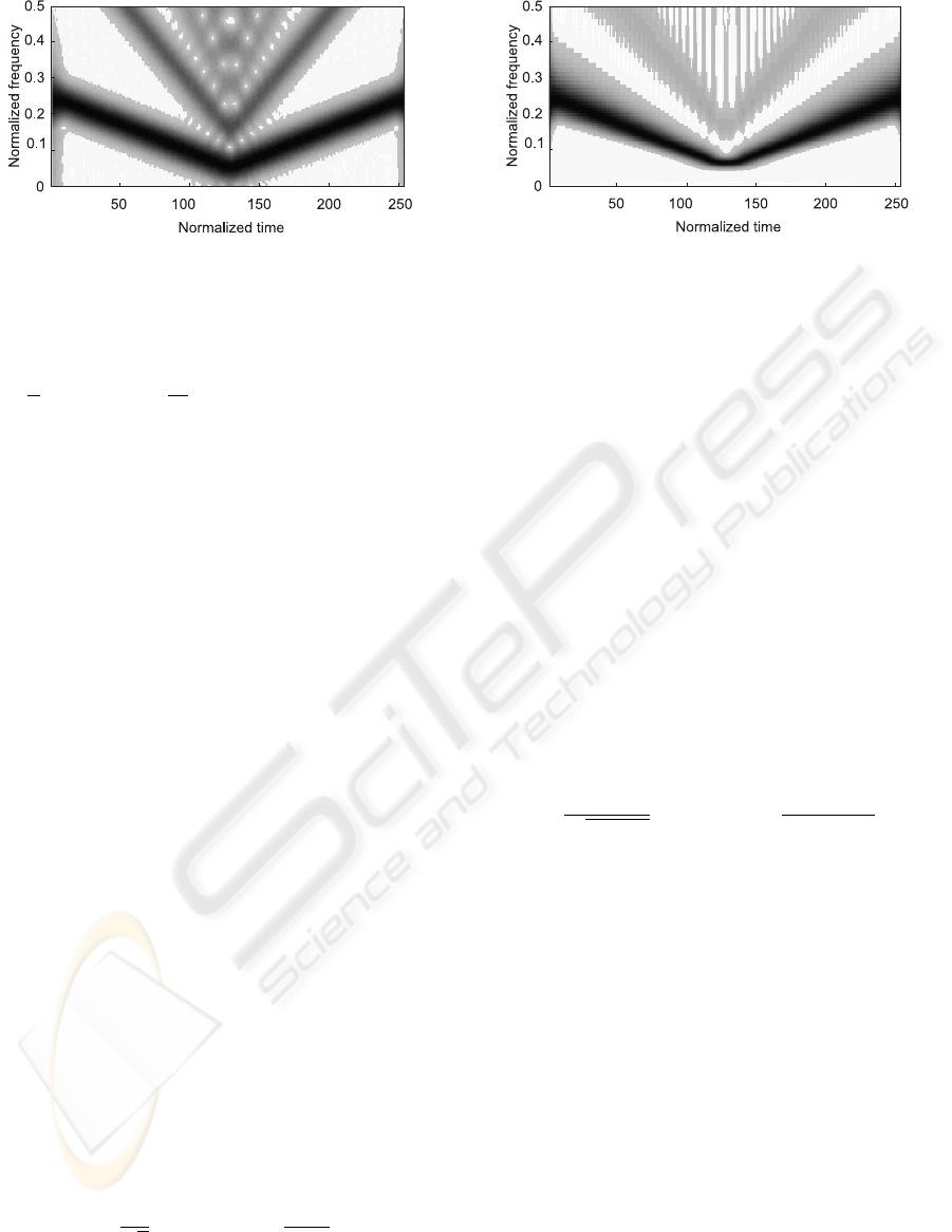
Figure 3: STFT based time-frequency representation of
test-signal sampled by crossing 7 levels.
within time interval Θ), the STFT based TFR on the
uniformly spaced time-frequency grid with frequency
step
1
Θ
and time step
1
2Ω
can be calculated as
T F R
ST F T
(k, m)
=
N
X
n=1
x
n
w
∗
(k/2Ω − t
n
) exp(−j2πt
n
m/Θ)
.
(12)
The expression (12) uses the general form of DFT, in
which the restriction, that requires the uniform spac-
ing of samples x
n
= nT , can be ignored. To examine
what happens if this expression is used for analysis
of level-crossing samples, the single chirp (parame-
ters of it will be described in the Section 6) is chosen
as a test-signal. The Fig.3 illustrates the fact that in
addition to the true component, spurious components
appear at the higher odd harmonics. These artifacts
are due to the use of LCS approach for signal with
regularities in the waveform. The additional source
of artifacts can be the absence of the orthogonality of
transformation functions exp(−j2πt
n
m/Θ) if t
n
are
not placed uniformly.
A well-known problem inherent in STFT is the in-
verse relationship between time and frequency reso-
lutions. Extension of the window’s w(t) length im-
proves the frequency resolution, but at the same time
degrades the temporal selectivity. To overcome this
difficulty of short time Fourier transform, alternative
methods of time-frequency analysis have been devel-
oped. The two most popular of them are a wavelet
transform and a Wigner-Ville distribution.
3.2 Wavelet Transform
The wavelet transform of a continuous-time signal
x(t) is defined as
W T (t, a) =
1
√
a
Z
∞
−∞
x(τ)h
∗
t − τ
a
dτ, (13)
where a is the scaling factor and h(t) is the so-called
analyzing wavelet. The time-frequency version is ob-
tained by making the substitution a = f
0
/f. The
Figure 4: WT based time-frequency representation of test-
signal sampled by crossing 7 levels.
analysis can be viewed as a filter bank comprising
bandpass filters with bandwidths proportional to fre-
quency. The multi-resolution nature of wavelet analy-
sis leads to some limitations. Wavelet transform uses
a scaling profile such that frequency resolution de-
creases at high frequencies, and temporal resolution
decreases at low frequencies. While this choice of
scaling leads to nice mathematical structures and al-
gorithms, there is no physical reason to assume that it
corresponds to natural structure behavior. For discrete
WT, in order to get the best performance of analy-
sis, the time- and scale-sampling grid often should be
considerably over-sampled, that introduces the redun-
dancy in the TFR.
The general form of time-frequency representation
based on discrete wavelet transform can be expressed
as
T F R
W T
(k, m)
=
1
p
f
0
Θ/m
N
X
n=1
x(t
n
)h
∗
k/2Ω − t
n
f
0
Θ/m
.
(14)
Such a notation enables the processing of both uni-
formly and non-uniformly sampled data. The nice
mathematical feature of WT for equidistantly spaced
samples states: for any k and a = 2
m
(k, m ∈ Z)
the {h(t
h
)}
(m,k)
is a subset of one discreet wavelet,
which is uniformly sampled at the sampling fre-
quency of the signal. In the case of non-equidistantly
spaced samples this property is lost, because the val-
ues of wavelet h(t) have to be calculated at different
points set {t
h
}
(m,k)
for each scaling factor a (or fre-
quency of analysis f = f
0
/a). Due to this fact, the
computation complexity of WT in the non-uniform
sampling case considerably exceeds the complexity
of the uniform sampling case.
The time-frequency representation obtained by
(14), if level-crossing sampling is used, is demon-
strated in Fig.4. It shows the reduction of the temporal
resolution in the low frequency region and diminished
spectral resolution in the high frequency region. The
PROCESSING OF NON-STATIONARY SIGNAL USING LEVEL-CROSSING SAMPLING
173

additional artifacts appear as well.
3.3 Wigner-Ville Distribution
Time-frequency analysis, based on the use of Wigner-
Ville function, is defined as
W V D(t, f)
=
Z
∞
−∞
x
t +
τ
2
x
∗
t −
τ
2
exp(−j2πfτ)dτ.
(15)
It provides high-resolution representation in time and
in frequency for mono-component signals. However,
if the signal consists of several subcomponents, ad-
ditional interference or cross-terms appear due to the
quadratic nature of kernel and non-linear properties
of it. In order to mitigate this deleterious effect, a va-
riety of modified kernels have been introduced. One
way to remove the interference is by smoothing the
time-frequency plane, but this will be at the expense
of decreased resolution in both time, and frequency.
A promising approach of how to suppress cross-terms
and improve resolution is the use of signal-dependent
kernels (Baraniuk and Jones, 1993).
A discrete form of the Wigner-Ville distribution
(WVD) can be expressed as
T F R
W V D
(k, m)
= 2
N
X
n=1
x(k/2Ω + t
n
)x
∗
(k/2Ω − t
n
)
·exp(−j4πt
n
m/Θ)|.
(16)
The necessity of knowing signal values at time in-
stants τ + t
n
and τ − t
n
for all n =
1, N leads
to the fact that the expression (16) can be used only
for uniform and specifically regular sampling series.
Therefore it is impossible to use the WVD approach
for processing data captured by the level-crossings.
4 ENHANCEMENTS OF DFT
It can be concluded from the discussion above, that
the most useful approach for practical applications
using the level-crossing sampling is based on STFT.
However it has to be enhanced and adjusted to the
LCS to suppress the presence of spurious compo-
nents.
The key operation of discrete STFT is the DFT
algorithm, which is applied to the windowed signal
samples. Thus the STFT enhancement can be reduced
to the development of DFT-like methods, which take
into account LCS features. The level-crossing sam-
pling principle provides not only samples at certain
events, but also the rule that the signal between two
sampling instants does not cross any quantization
level. This information can be exploited in the pro-
cessing. The proposed idea is to minimize the error
between the original signal and that reconstructed by
the Fourier series, not only at sampling time instants,
but also between them with the same accuracy. The
problem lies in the fact that the reconstruction error
can be obtained only at the time moments in which
the signal samples are known.
Basing on the Fourier series the signal waveform
can be reconstructed from its spectral estimates by the
following formula
ˆx(t) =
X
m
X
m
exp(j2πtf
m
), t ∈ [0, Θ], (17)
where X
m
are Fourier coefficients at frequencies
f
m
= m/Θ. If the original continues-time signal is
x(t), the reconstruction error is
ε(t) = x(t) − ˆx(t), (18)
and the following minimization task
Z
Θ
0
|ε(t)|
2
dt → min (19)
can be established on the understandings, that the sig-
nal values are known only at sampling points, and the
reconstructed signal is defined by (17). The problem
(19) has to be resolved with respect to the coefficients
{X
m
}. Two approaches can be considered: the first
one is based on setting up the continuous time sig-
nal by interpolation of known samples, while the sec-
ond approach, which minimizes the continuous time
reconstruction error, is based on the interpolation of
error samples.
4.1 Signal Interpolation
If signal samples {x
n
} are interpolated within the
time interval [0, Θ], the problem (19) can be rewrit-
ten as
Z
Θ
0
˜x(t) −
X
m
X
m
exp(j2πtf
m
)
2
dt → min,
(20)
where ˜x(t) is the interpolated signal. To find the min-
imum, all the individual derivatives of X
m
have to be
considered as being equal to zero. Taking into account
that {exp(j2πf
m
t)} is a set of orthogonal functions
into interval [0, Θ] if frequencies f
m
= m/Θ, after
some algebra the following formula for X
(x)
m
(
(x)
de-
notes that signal samples are interpolated) estimation
can be obtained:
X
(x)
m
=
1
Θ
Z
Θ
0
˜x(t) exp(−j2πtf
m
)dt. (21)
SIGMAP 2006 - INTERNATIONAL CONFERENCE ON SIGNAL PROCESSING AND MULTIMEDIA
APPLICATIONS
174

The expression (21) is similar to the formula for the
calculation of the Fourier series coefficients for signal
˜x(t).
Signal interpolation can easily be done by connect-
ing the samples with polynomials p
k
n
(t) of order k as
˜x(t) =
P
n
p
k
n
(t), or a band-limited interpolation can
be performed using a sum of time-shifted sinc func-
tions.
If signal samples are interpolated with zero-order
polynomials (piece-wise constant line changing value
at midpoints between samples):
X
(x0)
m
=
N
X
n=1
x
n
Z
t
n
+t
n+1
2
t
n
+t
n−1
2
exp(j2πf
m
t)dt
=
j
2πf
m
N
X
n=1
x
n
exp(j2πf
m
t
n
)
· (1 − exp(−j2πf
m
∆t
′
n
)),
(22)
where ∆t
′
n
= (t
n+1
− t
n−1
)/2, t
0
= 0, t
N+1
= Θ.
For piece-wise linear interpolation the polynomial
p
1
n
(t) = α
n
(t − t
n
) + x
n
can be used, where α
n
=
∆x
n
/∆t
n
, ∆x
n
= x
n
− x
n−1
, ∆t
n
= t
n
− t
n−1
,
which gives:
X
(x1)
m
= X
(x0)
m
+
1
(2πf
m
)
2
N
X
n=1
α
n
exp(j2πf
m
t
n
)
· (1 − exp(−j2πf
m
∆t
n
)) +
j
2πf
m
N
X
n=1
α
n
∆t
n
· exp(j2πf
m
t
n
) exp(−j2πf
m
∆t
n
).
(23)
Band-limited interpolation of samples can be de-
scribed as:
˜x
(sinc)
(t) =
K
X
k=0
c
k
sinc(2Ωt − k). (24)
In this case DFT transform gives:
X
(sinc)
m
=
K
X
k=0
c
k
exp(−jπf
m
k/Ω), (25)
where c
k
are coefficients that can be found from a lin-
ear equation system
x
n
=
K
X
k=0
c
k
sinc(2Ωt
n
− k). (26)
Such an approach, besides the complexity of DFT,
also requires the solution of linear system with N
equations and with K +1 unknowns. Interpolation by
sinc functions can be effectively done for the station-
ary signal and if the gaps between samples do not ex-
ceed 1/2Ω. In this case the appropriate width of func-
tion can be fixed. However, for the non-stationary sig-
nal, the sinc functions should be stretched and time-
shifted in accordance with instantaneous signal band-
width and local sampling density.
4.2 Error Interpolation
Like the interpolation of signal samples, the
continuous-time reconstruction error function ˜ε(t)
can be constructed from its values ε
n
= x
n
− ˆx
n
, and
the problem (19) can be interpreted as minimization
of area under the function |˜ε(t)|
2
.
Using zero-order polynomial interpolation the min-
imization task becomes:
N
X
n=1
x
n
−
X
m
X
(ε0)
m
exp(j2πf
m
t
n
)
2
∆t
′
n
→ min .
(27)
After the derivation and some algebra the solution can
be expressed in the matrix form:
X
(ε0)
= Ψx(ΦΨ
T
)
−1
, (28)
where φ
mn
= exp(j2πf
m
t
n
), ψ
mn
= φ
mn
∆t
′
n
, and
·
T
, ·
−1
denotes the transpose and inverse operation of
matrix respectively.
The first-order polynomial interpolation of error
samples provides the problem, which looks like a sum
of two zero-order interpolation tasks:
1
2
N−1
X
n=1
|ε
n
|
2
∆t
n
+
N
X
n=2
|ε
n
|
2
∆t
n−1
)
!
→ min .
(29)
The solution is similar to the expression (28):
X
(ε1)
= (Ψ
′
x
′
+ Ψ
′′
x
′′
)(Φ
′
Ψ
′
T
+ Φ
′′
Ψ
′′
T
)
−1
,
(30)
where Φ
′
, Ψ
′
, x
′
and Φ
′′
, Ψ
′′
, x
′′
matrices are
formed from Φ, Ψ, x by using indexes n
′
=
1, N − 1
and n
′′
=
2, N respectively.
5 PROPOSED APPROACH
The proposed approach is based on the same time
windowing principle as in the STFT case. How-
ever, instead of general DFT more sophisticated meth-
ods are used, which have been described in the Sec-
tion 4. Enhanced algorithms have increased mathe-
matical complexity, particularly the error interpola-
tion case, because the solving of linear system with
N equations and M unknowns is required. M rep-
resents a number of frequencies in the Fourier series.
The equation system can be solved correctly, if the
number of samples is equal or greater than the number
of frequencies. The greater the N/M ratio, the higher
the stability of the solution. It has been shown, that,
using the level-crossing sampling approach, the num-
ber of samples depends on the signal properties. Rela-
tionships between the local sampling density and the
instantaneous upper spectral frequency of signal have
PROCESSING OF NON-STATIONARY SIGNAL USING LEVEL-CROSSING SAMPLING
175
been derived. Performing the time-frequency analy-
sis, these interdependencies can be exploited from an
other point of view. The bandwidth of analysis can
be limited using information about the local sampling
density. The number of frequencies, as well as the
dimensions of matrices vary with the time. For simu-
lations, which will follow in the next section, the anal-
ysis bandwidth is selected as a minimum value of two
frequencies: total bandwidth Ω or highest signal fre-
quency estimated from the sampling density:
Ω
a
(t) = min
N
w
(t)
2R
∆
T
w
+ Ω
∆
, Ω
, (31)
where N
w
(t) is the number of signal samples in the
time interval with length T
w
, and Ω
∆
is necessary to
ensure the coverage of actual signal bandwidth. The
frequencies of analysis are f
m
= m/Θ : |f
m
| ≤ Ω
a
.
6 SIMULATION RESULTS
The computer simulation has been carried out to
demonstrate the performance of approaches, which
have been developed for time-frequency analysis of
data captured by level-crossings. As a test-signal
a chirp has been selected, which in the first half
of observation diminishes from middle frequency to
low frequency region (down to the normalized fre-
quency 0.05), while in the second half rises back to
the normalized frequency 0.25. Seven quantization
levels have been placed equidistantly to cover the in-
put range of the test-signal. The observation time is
Θ = 256, and 536 samples in total are obtained.
Time-frequency representations calculated by
STFT and WT approaches have been already il-
lustrated in the Section 3 (see Fig.3 and Fig.4).
Let us inspect the enhanced algorithms, which are
based on interpolation (expressions (22) and (23)).
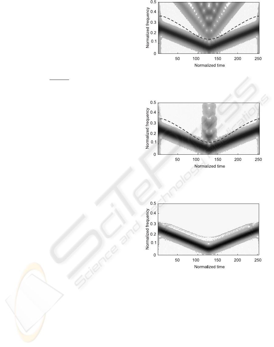
Fig.5 shows TFR obtained in the case, where time
windowed test-signal samples are interpolated by
zero-order polynomials. The spurious components
are attenuated, however the presence of them is still
observable. If the first-order polynomials are used
for interpolation, the result is slightly improved, but
the complexity of calculations is higher. Fig.6 shows
time-frequency representation of test-signal if error
samples are interpolated by zero-order polynomi-
als (28). The spurious harmonics are completely
suppressed, however other artifacts are observable
in the time region, where the frequency of chirp
is low. Reduction of the instantaneous frequency
results in the decreasing of local sampling density.
As the grid of temporal analysis and length of time
window w(t) are fixed, the number of the significant
samples can fall below the number of frequencies
of analysis. Such a situation causes the problem of
Figure 5: STFT approach in combination with zero-order
interpolation of signal samples (dashed line shows instanta-
neous bandwidth estimate from local sampling density).
Figure 6: STFT approach in combination with zero-order
interpolation of error samples (dashed line shows instanta-
neous bandwidth estimate from local sampling density).
Figure 7: TFR of test-signal if approach of varying the
range of analysis is used.
matrix inversion quality and leads to the appearance
of artifacts. The use of interpolation by first-order
polynomials does not have an impact on this effect.
To improve the quality of TFR in the region, where
sampling density is low, the bandwidth of analysis has
been cut down according to the expression (31). The
estimated bandwidth of signal is illustrated in Fig.6
and Fig.5 by dashed line (Ω
∆
= 0.1). The coher-
ence between the sampling density of a signal and
the frequency range of an analysis gives several ben-
efits - the stability of the algorithm is increased, the
complexity of calculations is decreased and the pres-
SIGMAP 2006 - INTERNATIONAL CONFERENCE ON SIGNAL PROCESSING AND MULTIMEDIA
APPLICATIONS
176

ence of artifacts is eliminated. Fig.7 demonstrates the
time-frequency representation obtained by the algo-
rithm based on the expression (28) in the case, where
the number of analysis frequencies are varied accord-
ing to the sampling density. The chirp can be tracked
without any presence of artifacts.
7 CONCLUSION
The processing of non-stationary signal using level-
crossing sampling approach has been investigated.
On the one hand, such a sampling strategy provides
several interesting properties - signal to quantization
noise ratio does not depend on the number of quan-
tization bits, local sampling density reflects the in-
stantaneous bandwidth of signal, etc. On the other
hand, the captured samples are placed non-uniformly
and that requires rethinking of the processing method-
ology. The classical approaches of time-frequency
analysis have been discussed. Time-frequency repre-
sentations have been obtained using general forms of
them, which are suitable also for processing of non-
uniformly sampled signals. The simulation shows
that the main drawback of STFT is the appearance of
spurious components, while wavelet transform gives
low spectral resolution at high frequencies and low
temporal resolution at low frequencies.
Several enhancements have been proposed, which
are based on the idea of minimizing the error be-
tween the original signal and that reconstructed by
the Fourier series, not only at sampling time instants,
but also between them with the same accuracy. The
problem lies in the fact that the original signal values
are known only at sampling instants. One solution is
based on the consideration, that the continuous time
signal is constructed by interpolation of known sig-
nal samples. The expressions for zero-order and first
order polynomial interpolation as well as for band-
limited interpolation with sinc functions have been
established. The other approach is to interpolate the
error samples in the same manner.
Simulation results show the improvement of TFRs
if enhanced algorithms are used instead of classical
ones. Additional benefits can be gained if the band-
width of analysis is varied along the time axis accord-
ing to changes in local sampling density: the artifacts
are removed, the complexity of calculations can be
decreased. The common drawback of STFT based
methods is restrictions on the resolution. Extension of
the windows w(t) length improves the frequency res-
olution but at the same time degrades the temporal se-
lectivity. To overcome this rule, the signal-dependent
transformation described in (Greitans, 2005) can be
used. Due to the limited size of the paper, this method
is not discussed above, however the TFR obtained by
Figure 8: TFR of test-signal if signal-dependent transfor-
mation is used.
signal-dependent algorithm is shown in the Fig.8 for
the illustration. The increased resolution is achieved
by adapting the transformation functions to the local
spectral characteristics of the signal. As it is being
done in an iterative way, the mathematical complex-
ity is higher than for STFT based algorithms.
The proposed approach of processing non-
stationary signals using level-crossing sampling is
attractive for clock-less designs, which are now re-
ceiving increasing interest. Their advantages can play
a significant role in future electronics’ development.
REFERENCES
Akay, M., editor (1998). Time frequency and wavelets in
biomedical signal processing. IEEE Press.
Baraniuk, R. G. and Jones, D. L. (1993). A signal-
dependent time-frequency representation: Optimal
kernel design. IEEE Trans. Signal Proc., 41(4):1589–
1602.
Chui, C. K. (1992). Wavelet Analysis and its Applications.
Academic Press, Boston, MA.
Cohen, L. (1995). Time-frequency analysis. Prentice-Hall.
E. Allier, G. Sicard, L. F. and Renaudin, M. (2003). A new
class of asynchronous a/d converters based on time
quantization. In Proc. of International Symposium on
Asynchronous Circuits and Systems ASYNC’03, pages
196–205, Vancouver, Canada.
Ellis, P. H. (1959). Extension of phase plane analysis to
quantized systems. IRE Transactions on Automatic
Control, AC(4):43–59.
Gabor, D. (1946). Theory of communication. Journal of
the IEE, 93(3):429–457.
Greitans, M. (2005). Spectral analysis based on signal de-
pendent transformation. In Proc. of the International
Workshop on Spectral methods and multirate signal
processing, pages 179–184, Riga, Latvia.
Hauck, S. (1995). Asynchronous design methodologies: An
overview. Proc. of the IEEE, 83(1):69–93.
Mark, J. W. and Todd, T. D. (1981). A nonuniform sam-
pling approach to data compression. IEEE Trans. on
Comm., 29(1):24–32.
PROCESSING OF NON-STATIONARY SIGNAL USING LEVEL-CROSSING SAMPLING
177
