
OPTIMIZED GAUSS AND CHOLESKY ALGORITHMS FOR
USING THE LMMSE DECODER IN MIMO/BLAST SYSTEMS
WITH FREQUENCY-SELECTIVE CHANNELS
Reduced-complexity Equalization
João Carlos Silva, Nuno Souto, Francisco Cercas, António Rodrigues
Instituto Superior Técnico/IT, Torre Norte 11-11, Av. Rovisco Pais 1, 1049-001 Lisboa, Portugal
Rui Dinis, Sérgio Jesus
CAPS, Av. Rovisco Pais 1,1049-001 Lisboa, Portugal
Keywords: MMSE Equalizer, Gauss, Cholesky, MIMO, W-CDMA.
Abstract: The LMMSE (Linear Minimum Mean Square Error) algorithm is one of the best linear receivers for DS-
CDMA (Direct Sequence-Code Division Multiple Access). However, for the case of MIMO/BLAST
(Multiple Input, Multiple Output / Bell Laboratories Layered Space Time), the perceived complexity of the
LMMSE receiver is taken as too big, and thus other types of receivers are employed, yielding worse results.
In this paper, we investigate the complexity of the solution to the LMMSE and the Zero-Forcing (LMMSE
without noise estimation) receiver’s equations. It will be shown that the equation can be solved with
optimized Gauss or Cholesky algorithms. Some of those solutions are very computationally efficient and
thus, allow for the usage of the LMMSE in fully-loaded MIMO systems.
1 INTRODUCTION
Digital communication using MIMO, sometimes
called a “volume-to volume” wireless link, has
recently emerged as one of the most significant
technical breakthroughs in modern communications.
Just a few years after its invention the technology is
already part of the standards for wireless local area
networks (WLAN), third-generation (3G) networks
and beyond.
MIMO schemes are used in order to push the
capacity and throughput limits as high as possible
without an increase in spectrum bandwidth, although
there is an obvious increase in complexity. For N
transmit and M receive antennas, we have the
capacity equation (Foschini, 1998), (Telatar, 1999)
2
log det I '
EP M
CHH
N
ρ
⎛⎞
⎛⎞
=+
⎜⎟
⎜⎟
⎝⎠
⎝⎠
b/s/Hz (1)
where H is the channel matrix, H’ is the
transpose-conjugate of H and ρ is the SNR at any
receive antenna. (Foschini, 1998) and (Telatar, 1999)
both demonstrated that the capacity grows linearly
with m=min(M,N), for uncorrelated channels.
Therefore, it is possible to augment the
capacity/throughput by any factor, depending on the
number of transmit and receive antennas. The
downside to this is the receiver complexity,
sensitivity to interference and correlation between
antennas, which is more significant as the antennas
are closer together. For a 3G system, for instance, it
is inadequate to consider more than 2 or 4 antennas at
the UE (User Equipment)/ mobile receiver.
Note that, unlike in CDMA where user’s
signatures are quasi-orthogonal by design, the
separability of the MIMO channel relies on the
presence of rich multipath which is needed to make
the channel spatially selective. Therefore, MIMO can
be said to effectively exploit multipath.
The receiver for such a scheme is obviously
complex; due to the number of antennas, users and
multipath components, the performance of a simple
RAKE/ MF (Matched Filter) receiver (or enhanced
schemes based on the MF) always introduces a
200
Carlos Silva J., Souto N., Cercas F., Rodrigues A., Dinis R. and Jesus S. (2006).
OPTIMIZED GAUSS AND CHOLESKY ALGORITHMS FOR USING THE LMMSE DECODER IN MIMO/BLAST SYSTEMS WITH FREQUENCY-
SELECTIVE CHANNELS - Reduced-complexity Equalization.
In Proceedings of the International Conference on Wireless Information Networks and Systems, pages 200-208
Copyright
c
SciTePress

significant amount of noise, that doesn’t allow for the
system to perform at full capacity. Thus being, the
LMMSE receiver was considered for such cases,
acting as an equalizer.
The structure of the paper is as follows. In
Section II, the LMMSE receiver for MIMO with
multipath is introduced. Section III presents the
proposed optimizations to the standard methods of
Gauss and Cholesky. In section IV an approximate
method based in the Cholesky way is discussed, and
conclusions are drawn in Section V.
2 LMMSE RECEIVER
A standard model for a DS-CDMA system with K
users (assuming 1 user per physical channel) and L
propagation paths is considered. The modulated
symbols are spread by a Walsh-Hadamard code with
length equal to the Spreading Factor (SF). The signal
on a MIMO-BLAST system with N
TX
transmit and
N
RX
receive antennas, at one of the receiver’s
antennas, can be expressed as:
A standard model for a DS-CDMA system with K
users (assuming 1 user per physical channel) and L
propagation paths is considered. The symbols
(QPSK/16QAM) are spread by a Walsh-Hadamard
code with length equal to the Spreading Factor (SF).
The received signal on a MIMO system with N
TX
transmit and N
RX
receive antennas on one of the
receiver’s antennas can be expressed as:
()
1,, ,,
111
() ( )* () ()
TX
N
NK
n
v RX ktx ktx k ktxrx
ntxk
rt A b s t nT c t nt
=
===
=−+
∑∑∑
(2)
where N is the number of received symbols,
,ktx k
A
E=
, E
k
is the energy per symbol,
()
,
n
ktx
b
is the
n-th transmitted data symbol of user k and transmit
antenna tx, s
k
(t) is the k-th user’s signature signal
(equal for all antennas), T denotes the symbol
interval, n(t) is a complex zero-mean AWGN with
variance
2
σ
,
()
,, ,, , ,
1
() ( )
L
n
ktxrx ktxrxl kl
l
ct c t
δ
τ
=
=−
∑
is the
impulse response of the k
-
th user’s radio channel,
c
k,tx,rx,l
is the complex attenuation factor of the k-ths
user’s l-th path of the link between the tx-th and rx-
th antenna,
,kl
τ
is the propagation delay (assumed
equal for all antennas) and (*) denotes convolution.
The received signal on can also be expressed as:
()
1 ,,,, ,
1111
() () ( ) ()
TX
N
NKL
n
vRX ktxktxktxrx k kl
ntxk l
rt A b c tst nT nt
τ
=
====
=−−+
∑∑∑∑
(3)
Using matrix algebra,
v
rSCAbn=+
, where S, C and
A are the spreading, channel and amplitude matrices
respectively. The spreading matrix S has dimensions
(
)
(
)
R
X MAX RX RX
SF N N N K L N N
τ
⋅⋅ + ⋅ × ⋅⋅⋅
(τ
max
is
the maximum delay of the channel’s impulse
response, normalized to number of chips), and is
composed of sub-matrices S
RX
in its diagonal for
each receive antenna
RX
RX=1 RX=N
S=diag(S , ,S )…
. Each
of these sub-matrices has dimensions
(
)
(
)
MAX
SF N K L N
τ
⋅
+×⋅⋅
, and are further
composed by smaller matrices S
L
n
, one for each bit
position, with size
(
)
(
)
MAX
SF K L
τ
+
×⋅
. The S
RX
matrix structure is made of
( )() ( )()
L
RX,n n
SF ( 1) K L SF (N-n) K L
RX RX,1 RX,N
S=0 ,S,0
S=S , ,S
T
n⋅− × ⋅ ⋅ × ⋅
⎡
⎤
⎣
⎦
⎡⎤
⎣⎦
…
The S
L
matrices are made of
K
L⋅
columns;
L
n col(k=1,l=1),n col(k=1,l=L),n col(k=K,l=L),n
S=S , ,S , ,S
⎡
⎤
⎣
⎦
……
. Each
of these columns is composed of
()
()
()
col(KL),n 1
1 delay(L)
1()
S=0 , (),0
MAX
T
nSF
delay L
spread K
τ
×
×
×−
⎡
⎤
⎣
⎦
,
where spread
n
(K) is the combined spreading &
scrambling for the bit n of user K.
These S
L
matrices are either all alike if no long
scrambling code is used, or different if the
scrambling sequence is longer than the SF. The S
L
matrices represent the combined spreading and
scrambling sequences, conjugated with the channel
delays. The shifted spreading vectors for the
multipath components are all equal to the original
sequence of the specific user.
1,1,1, ,1,1,
1,1, , ,1, ,
1, ,1, , ,1,
1, , , , , ,
nKn
Ln K Ln
L
n
SF n K SF n
SF L n K SF L n
SS
SS
S
SS
SS
⎡
⎤
⎢
⎥
⎢
⎥
=
⎢
⎥
⎢
⎥
⎢
⎥
⎣
⎦
Note that, in order to correctly model the multipath
interference between symbols, there is an overlap
between the S
L
matrices, of τ
MAX
.
The channel matrix
C is a
(
)
(
)
RX TX
K
LNN KN N
⋅
⋅⋅ × ⋅ ⋅
matrix, and is
composed of RX sub-matrices, each one for a RX
antenna
RX
RR
1RX=N
C= C , , C
T
RX =
⎡
⎤
⎣
⎦
…
. The diagonals of
each C
R
matrix are composed of N C
KT
matrices.
1,1
,1
1,
,
RX
RX
KT
KT
N
KT
N
KT
NN
C
C
C
C
C
⎡
⎤
⎡
⎤
⎢
⎥
⎢
⎥
⎢
⎥
⎢
⎥
⎢
⎥
⎢
⎥
⎣
⎦
⎢
⎥
=
⎢
⎥
⎢
⎥
⎡
⎤
⎢
⎥
⎢
⎥
⎢
⎥
⎢
⎥
⎢
⎥
⎢
⎥
⎢
⎥
⎣
⎦
⎣
⎦
Each C
KT
matrix is
(
)
(
)
TX
KL KN⋅× ⋅
, and
represents the fading coefficients for each path, user
and TX antenna, for the current symbol and RX
OPTIMIZED GAUSS AND CHOLESKY ALGORITHMS FOR USING THE LMMSE DECODER IN MIMO/BLAST
SYSTEMS WITH FREQUENCY-SELECTIVE CHANNELS - Reduced-complexity Equalization
201

antenna. The matrix structure is made up of further
smaller matrices along the diagonal
(
)
KT T T
K=1 K=K
C=diagC , ,C…
, with C
T
of dimensions
TX
L
N×
, representing the fading coefficients for the
user’s multipath and tx-th antenna component.
1,1,1 ,1,1
1, ,1 , ,1
1,1, ,1,
1, , , ,
TX
TX
TX
TX
N
LNL
KT
KNK
LK N LK
CC
CC
C
CC
CC
⎡⎤
⎢⎥
⎢⎥
⎢⎥
⎢⎥
=
⎢⎥
⎢⎥
⎢⎥
⎢⎥
⎢⎥
⎣⎦
The A matrix is a diagonal matrix of
dimension
(
)
TX
K
NN⋅⋅
, and represents the
amplitude of each user per transmission antenna and
symbol,
(
)
TX TX TX
1,1,1 N ,1,1 N ,K,1 N ,K,N
A=diag A , , A , , A , , A…… …
.
Vector
b represents the information symbols. It has
length
(
)
TX
KN N⋅⋅
, and has the following
structure
TX TX TX
1,1,1 N ,1,1 1,K,1 N ,K,1 N ,K,N
b= b , ,b , ,b , ,b , ,b
T
⎡⎤
⎣⎦
……… …
.
Note that the bits of each TX antenna are grouped
together in the first level, and the bits of other
interferers in the second level. This is to guarantee
that the resulting matrix to be inverted has all its
non-zeros values as close to the diagonal as possible.
Also note that there is usually a higher correlation
between bits from different antennas using the same
spreading code, than between bits with different
spreading codes.
Finally, the
n vector is a
(
)
R
XRXMAX
NSFN N
τ
⋅⋅ + ⋅
vector with noise components to be added to the
received vector r
v
, which is partitioned by N
RX
antennas,
RX RX
v 1,1,1 1,SF,1 N,1,1 N,SF+ ,1 N,1,N N,SF+ ,N
r = R , ,R , ,R , ,R , ,R , ,R
MAX MAX
T
ττ
⎡⎤
⎣⎦
……… … …
The MMSE algorithm yields the symbol estimates,
y
MMSE
, which should be compared to vector b,
(
)
H
MF
H
ySCArv
R
SS
=
=⋅
,
(
)
1
2
MMSE MF
H
yEMy
E
MACRCA I
σ
−
=
=+
(4)
where
2
σ
is the noise variance of n, y
MF
is the
matched filter output and EM is the Equalization
Matrix (cross-correlation matrix of the users’
signature sequences after matched filtering, at the
receiver).
The expected main problem associated with such
scheme is the size of the matrices, which assume
huge proportions. Due to the multipath causing
Inter-Symbolic Interference (ISI), the whole
information block has to be simulated at once,
requiring the use of a significant amount of memory
and some computing power for the algebraic
operations, with emphasis on the inversion of the
EM in the MMSE algorithm.
Matrix Reordering
Matrix reordering is used in order to simplify the
solving of the MMSE equation. While in the original
version the
SCA matrix is devised in such a way as
to make the received vector is divided per receive
antenna in order to make the system matrices more
perceivable, the reordering of the structure of the
SCA matrix is done solely to simplify processing.
Replacing:
()
reord=TSCA
;
2
σ
=NI
;
ˆ
M
MSE
=dy
and ()
V
reord
=
er in the MMSE
equation we obtain a simpler version:
1
()
HH−
=+
d
TT N Te
where
(
)
reord x
represents a line-reordering of
vector or matrix
x where the lines of each antenna
were intercalated with the propose of making a more
compact and almost block-circulant matrix.
()
1
2
1
2
(1, :)
(1, :)
(1, :)
(,:)
(,:)
(,:)
TX
TX
TX
TX
TX N
TX
TX
TX N
reord
N
N
N
=
=
=
=
=
=
⎡
⎤
⎢
⎥
⎢
⎥
⎢
⎥
⎢
⎥
⎢
⎥
⎢
⎥
=
⎢
⎥
⎢
⎥
⎢
⎥
⎢
⎥
⎢
⎥
⎢
⎥
⎢
⎥
⎣
⎦
x
x
x
x
x
x
x
(6)
Figure 1(a) shows the reordering result for a two
antennas matrix. For high SNRs equation (5)
becomes the Zero-Forcing detector equation:
1
()
HH−
=dTTTe (7)
Since usually
MAX
SF
τ
≤
, the
H
TT product
results in a square matrix with the structure
presented in Figure 1(b) with:
2
TX
aKN= and
TX
nKNN
=
. It can be shown that
H
TTis a
positive definite Hermitian matrix. Earlier works
(Vollmer, 2001), (Machauer, 2001), dealt only with
the Zero-Forcing detector equation for constant
channel situations. Here the validity of those
algorithms for unsteady channels situations will be
evaluated. New algorithms for unsteady channel
situations will be proposed and some optimizations
will be also introduced and presented in pseudo-code
form. Finally, all the algorithms will be adapted to
the LMMSE detector.
WINSYS 2006 - INTERNATIONAL CONFERENCE ON WIRELESS INFORMATION NETWORKS AND SYSTEMS
202
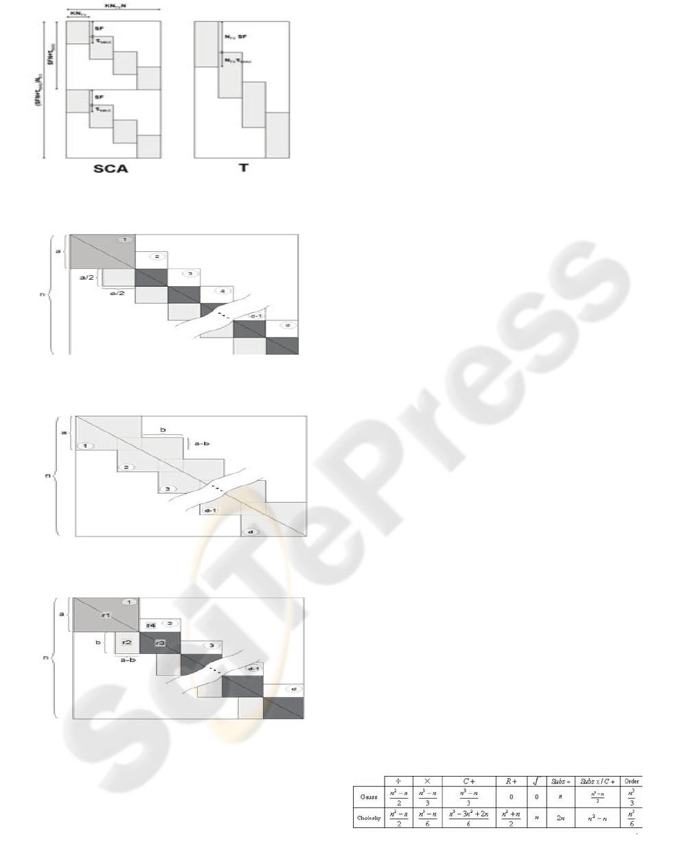
Figure 1: Line reordering sample for N
TX
= 2.
Figure 2: Typical correlation matrix.
Figure 3: Generalized equalization matrix.
Figure 4: Optimized Gauss algorithm.
3 GAUSS AND CHOLESKI
ALGORITHMS
Equation (7) can be written as an Ax=b system with
A being a positive definite Hermitian matrix, where
H
A
=
TT,
x
=
d and
H
b = Te. It can be solved
for
x using the Gauss elimination or the Cholesky
algorithm.
We are interested in solving the
Ax=b system for a
particular
b vector only, so there is no need to invert
the
A matrix. The Gauss elimination can be used to
transform the
Ax=b system in a Ux=b’ where U is an
upper triangular matrix and then
x can be obtained
by direct substitution. The Cholesky method is a
little bit more complex: first
A is factorized in
A=U
H
U by the Cholesky algorithm, then U
H
Ux=b
can be decomposed in
U
H
c=b and Ux=c; these two
systems can be solved by direct substitution. The
Cholesky algorithm can save almost half of the
floating point operations needed in the Gauss
elimination because it takes advantage of the
symmetry of the
A matrix, but the Gauss elimination
is less complex and requires no square roots to be
calculated. Previous works (Noguet, 2004) have
successfully designed and implemented a real-time
hardware structure of the regular Cholesky
algorithm for the ZF joint-detection algorithm in the
UMTS/TDD context based on a SIMD structure
(Flynn, 1972) (systolic array). With the algorithms
presented in this paper a significant complexity
reduction can be expected, thereby reducing by a
great amount the size of the hardware structure,
alongside the cost and processing time. Table 1(a)
shows the number of floating point operations
required by both methods. The additions are
separated into real and complex (R+ and C+,
respectively). The extra operations wasted by the
Gauss algorithm are partially recovered in the
substitution phase, where the Cholesky method
requires the solution of two triangular systems and
hence twice the operations of the Gauss algorithm.
The number of operations required in this phase is
also included in Table 1(a).
The Order column presents the highest power of the
total number of operations considering each
multiplication-addition pair as a single operation.
Table 1: Number of floating operations needed to solve
the Ax=b system with standard Gauss algorithm.
OPTIMIZED GAUSS AND CHOLESKY ALGORITHMS FOR USING THE LMMSE DECODER IN MIMO/BLAST
SYSTEMS WITH FREQUENCY-SELECTIVE CHANNELS - Reduced-complexity Equalization
203
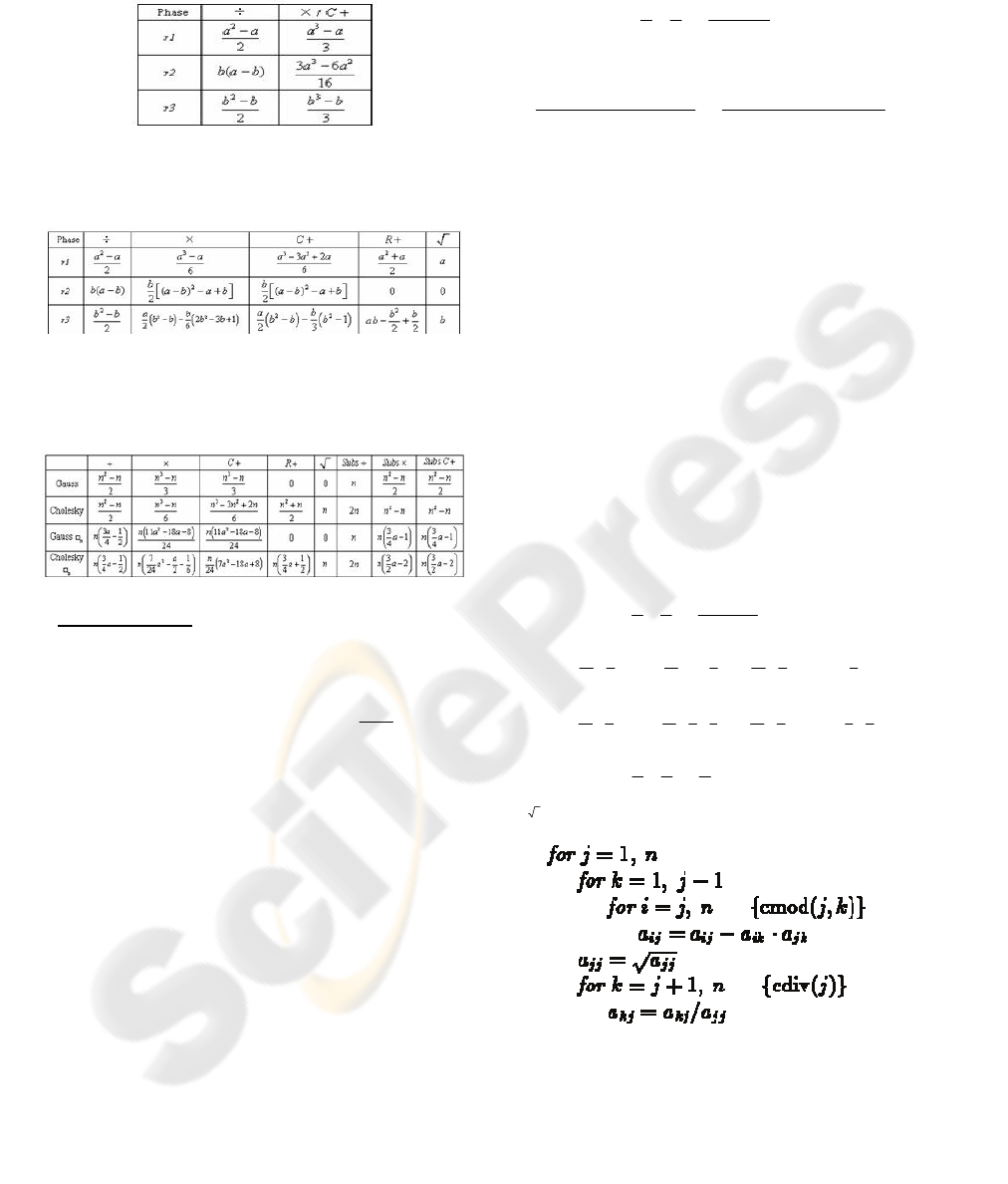
Table 2: Number of floating operations needed to solve
the Ax=b system with optimized Gauss algorithm.
Table 3: Number of floating operations needed to solve
the Ax=b system with optimized Cholesky algorithm.
Table 4: Number of floating operations needed to solve
the Ax=b system with optimized Cholesky algorithm;
special case when
/2ba=
.
Optimizations
A generic positive definite Hermitian matrix that is
nonzero only in equally overlapped squares centred
along the diagonal is represented in Figure 1(c). The
number of overlapped squares is
1
na
d
b
−
=+
. The
Gauss algorithm can be optimized for this type of
matrix by eliminating the operations involving zero
elements. The idea is presented in Figure 1(d). First,
the standard Gauss algorithm is applied to the r1
square sub-matrix. There is no need to change the r4
rectangle. Next step is the elimination of the r2
block using the last a-b pivots of r1 (the pivots are
the diagonal elements after the elimination phase).
During this phase r3 is updated. Finally the
standard algorithm is applied to r3. This process is
repeated until all blocks are updated. During this
process, as each line is updated, the correspondent
element of vector
b is simultaneously updated. Note
that the matrix diagonal is fully contained in the
diagonal squares.
Table 1(b) presents the number of floating point
operations required in each of the tree phases
described. The total number of operations can be
calculated from:
(
)
123
(1)
Gauss Opt Gauss r Gauss r Gauss r
NNdNN=+− +
(8)
Leading to:
1()
22 2
Gauss Opt
baab
Nna
÷
−
⎛⎞
=−−−
⎜⎟
⎝⎠
(9)
()
()
32 2
32 3
91816 1
928916
48 48
C
Gauss Opt Gauss Opt
NN
aabb
aab b
na
bb
×+
==
−+ −
−++
=−
(10)
A similar adaptation can be developed for the
Cholesky factorization algorithm. We will optimize
the column-Cholesky algorithm (presented in Figure
5) although similar results could be achieved for the
line version of that algorithm. Figure 6(a) sketches
such approach. In this case only the upper triangle
has to be accessed. First, the standard column-
Cholesky algorithm is applied to the r1 triangle. In a
second step the rectangle r2 is calculated accessing
only the elements of r2 and r1. In the next step, the
triangle r3 is computed using only elements of r2
and r3. Last two steps are repeated for all remaining
blocks, using always only elements of the last and
current block. As in the optimized Gauss algorithm,
the rectangular blocks do not contain the diagonal.
Table 1(c) presents the number of floating point
operations of the tree phases described. The total
number of operations can be calculated from:
(
)
123
(1)
Chol Opt Chol r Chol r Chol r
NNdNN=+− +
(11)
Leading to:
1()
22 2
Chol Opt
baab
Nna
÷
−
⎛⎞
=−−−
⎜⎟
⎝⎠
(12)
()
22 2
1
2(2)1
22 6 6 32 6
Chol Opt
aa b aa b
Nn b ba bb
×
⎛⎞⎛
⎞
⎛⎞
=−+++−−−+++
⎜⎟⎜
⎟
⎜⎟
⎝⎠
⎝⎠⎝
⎠
(13)
()
22 2
11
2(1)
22 623 32 62
C
Chol Opt
aa bb aa b
Nn b a bb
+
⎛⎞⎛
⎞
⎛⎞
= − + + ++ − − ++ +
⎜⎟⎜
⎟
⎜⎟
⎝⎠
⎝⎠⎝
⎠
(14)
1
()
22 2
R
Chol Opt
ba
N
na b a
+
⎛⎞
=
−+ + −
⎜⎟
⎝⎠
(15)
Chol Opt
N
n
=
(16)
Figure 5: Column oriented Cholesky factorization.
Both Gauss and Cholesky methods need final
substitution phases. These substitutions can also be
optimized since the resulting matrices have a
structure similar to the original
A matrix but with
WINSYS 2006 - INTERNATIONAL CONFERENCE ON WIRELESS INFORMATION NETWORKS AND SYSTEMS
204
nonzero elements only above (or below) the
diagonal, like shown in Figure 6(b).
The solution of a system
Ax=b with A having a
structure similar to the structure presented in Figure
6(b) requires one division for each line of the matrix
and one pair multiplication-addition for each
nonzero element. Since there are
()
()
()
2
2
1
22
ab
a
dad ab
⎛⎞
−
⎛⎞
⎜⎟
−−− −−
⎜⎟
⎜⎟
⎝⎠
⎝⎠
(17)
nonzero elements, the number of floating point
operations needed can be written:
Subs Opt
Nn
÷
=
(18)
()
1
22
C
Subs Opt Subs Opt
aa b
b
NNna
×+
−
⎛⎞
==−−−
⎜⎟
⎝⎠
(19)
We are interested in a special type of block-diagonal
positive definite Hermitian matrices, with
/2ba
=
,
like represented in Figure 6(b). Re-writing the above
equations for this special case and keeping only the
n-dependent terms (
na>>
), results in Table 1(d) As
can be seen, the optimized Cholesky algorithm can
save almost 30% of the number of operations
required for the optimized Gauss algorithm, despite
it increased complexity and need of square root
operations.
Figure 6: (a) Optimized Cholesky algorithm, (b) Gauss
elimination / Cholesky factorization resulting matrix
structure.
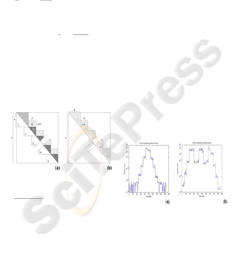
Partitioning
Partitioning the block-diagonal system Ax=b would
be very useful to reduce the number of floating point
operations needed to solve the system (if no overlap
is used; i.e., in good channel conditions) and also
could permit the introduction of parallelism is
algorithms that are intrinsically sequential, like the
algorithms presented in previous sections. In this
section we will discuss different partitioning
approaches.
Since A is block-diagonal and has generally
decreasing values as we get farther from its
diagonal, it is expected that it can be divided in
smaller matrices that produce smaller systems whose
combined solutions would approximate the solution
of the original system. Figure 7(a) presents a sample
solution of a system simply divided in 2 sub-systems
as sketched in Figure 8(a). Note that there are two
m × m blocks completely ignored at the middle of
the A matrix. Surprisingly the obtained maximum
error is only 12% of the exact solution. Figure 7(b)
shows the same data when the
A matrix is divided in
four slices. The maximum error level is
approximately the same as in the previous case, but
now we have three high error regions.
Although the error obtained with the last partitioning
method is not extremely high and appear only
around the division lines, much better results can be
attained if overlapping partitions are considered.
This proceeding is sketched in Figure 8(b). Each
slice overlaps the last in 2 × lap blocks (a lap being
the number of blocks that are discarded from each
overlapping side of each computed slice). Note that
the last slice can be smaller.
From each slice are obtained
(2)Dlapm−
values for
the solution vector x, except in the case of the first
and last slices, where
()Dlapm−
and
(( 1) )
M
LDlapm
−
−+
values are obtained
respectively.
As seen in Figure 7(a) and (c), the error level rises at
the beginning and end of each slice, so the
overlapping method should discard that values. In
each iteration are discarded lap × m values from the
beginning and lap × m values from the end, except
in the first end last slice, where are only discarded
the last lap × m and first lap × m values respectively.
Figure 7: Relative error obtained solving a no-overlap
partitioned system. (a) - M=192; m=12; D=8; v=10Km/h,
(b) - M=192; m=12; D=4; v=10Km/h.
OPTIMIZED GAUSS AND CHOLESKY ALGORITHMS FOR USING THE LMMSE DECODER IN MIMO/BLAST
SYSTEMS WITH FREQUENCY-SELECTIVE CHANNELS - Reduced-complexity Equalization
205
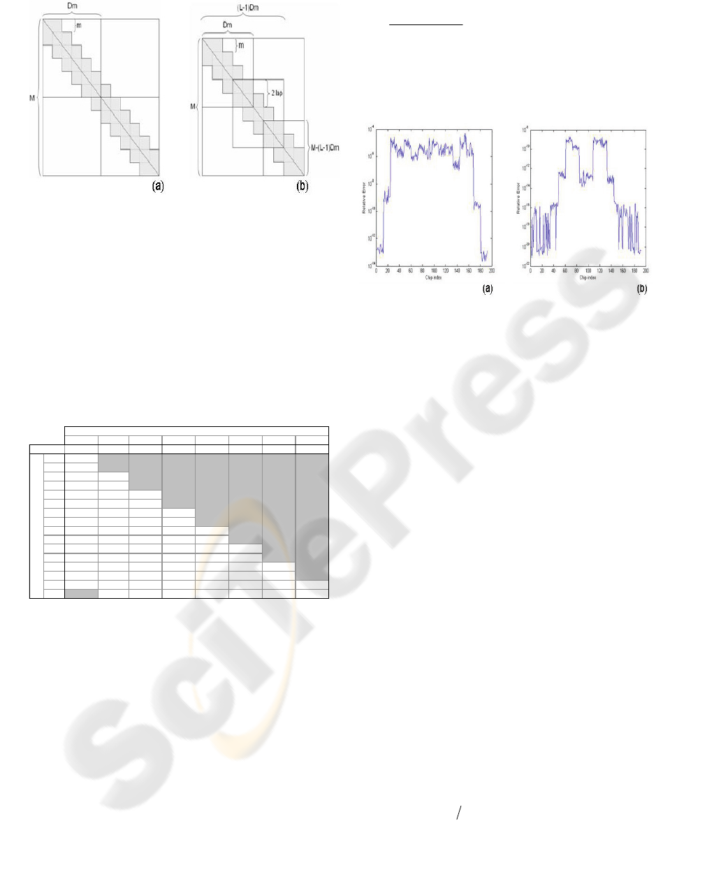
Figure 8: Partitioning (a) - without overlapping, (b) – with
overlapping.
An alternative to have a final slice with size smaller
than the early ones is to extend the b vector with
zeros until
/2
M
mlap−
becomes multiple
of
2Dlap−
. Several simulations were run for
different channel changing speeds. Similar results
were obtained for all matrices tested. Sample results
are presented in Table 2, for a 10Km/h condition.
Table 5: Maximum relative error for the partitioning
algorithm; v=10Km/h.
01234567
1.E+00 1.E-04 1.E-07 1.E-11 1.E-15 1.E-15 1.E-15 1.E-15
1 0.506
2 0.459
3 0.152 0.911
4 0.221 0.494
5 0.127 0.494 0.090
6 0.082 0.494 0.123
7 0.459 0.105 0.123 0.247
8 0.221 0.494 0.021 0.063
9 0.083 0.640 0.042 0.038 0.898
10 0.099 0.194 0.123 0.063 0.637
11 0.079 0.190 0.037 0.222 0.817 0.505
12 0.033 0.082 0.020 0.038 0.646 0.623
13 0.159 0.059 0.015 0.036 0.642 0.552 0.416
14 0.459 0.494 0.018 0.047 0.572 0.432 0.504
15 0.127 0.845 0.090 0.033 0.420 0.284 0.252 0.378
16 0.009 0.005 0.006 0.479 0.232 0.432 0.504
D
Factor:
lap
All the values presented should be multiplied by the
corresponding column factor to obtain the maximum
error of the partition algorithm relative to the exact
solution of the original Ax=b system. The column
for lap=0 corresponds to the lap less situation.
shows that the maximum error level depends almost
exclusively from the overlapping level, so the proper
overlapping can be easily selected just by knowing
the maximum error allowed in the real system. The
number of blocks D processed by each thread can be
selected from the total number of threads L that can
be executed simultaneously by the hardware, using
the relation:
/2
2
M
mlap
L
Dlap
⎡
⎤
−
=
⎢
⎥
−
⎢
⎥
, (20)
where
x
⎡
⎤
⎢
⎥
represents the smallest integer greater
than or equal to x. Some results of the relative error
obtained in an overlap system are portrayed in
Figure 9.
Figure 9: Relative error obtained solving an overlap
partitioned system (a) - D=4; lap=1; v=10Km/h, (b) - D=8;
lap=2; v=10Km/h.
4 PARTIAL CHOLESKI
APPROXIMATION
The Cholesky decomposition of block-Toeplitz
matrices is an upper (or lower) matrix approximately
block-Toeplitz with the same block size as the
original matrix. This means that the U matrix can be
approximated calculating only the first L block-rows
and assuming that the remaining block-rows are
identical to the last calculated block-row. Figure 7
shows this approach. Only the dark shaded part is
computed. The last computed block (marked as L) is
then repeated until the full matrix is completed. This
approximation is very effective when the channel is
constant.
Figure 8 shows the maximum relative error of the
system solution for each approximation level (L) i.e.
the number of calculated blocks, for different speeds
in a pedestrian A condition with 1 antenna.
As can be seen for a constant channel, calculating
only the first one or two blocks allows
approximations in the system solution with relative
error below 10
-4
or 10
-9
. This can be used to greatly
reduce the number of operations necessary to solve
the system. If only 2 blocks are calculated the
number of operations can be reduced approximately
by a factor of
an
. However, when the channel
changes, this approach can not be used regarding to
the high error level obtained (unless the channel
change is very slow).
WINSYS 2006 - INTERNATIONAL CONFERENCE ON WIRELESS INFORMATION NETWORKS AND SYSTEMS
206
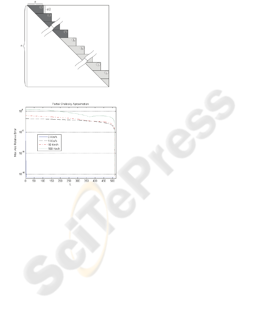
Figure 10: Partial Cholesky approximation.
Figure 11: Partial Cholesky approximation; (pedestrianA –
minimum load).
5 CONCLUSIONS
In this work where presented optimized versions of
the Gauss and Cholesky algorithms that can be used
in the solution of the equation of a zero-forcing or
LMMSE detector in MIMO/BLAST systems. Those
optimizations were based simply in the removal of
the unnecessary operations regarding the structure of
the involved matrices. It has the advantage of being
a velocity independent solution, unlike other
methods such as the Block-Fourier (Vollmer, 2001),
(Machauer, 2001). The benefit of parallel processing
can also be exploited for these methods, with the
introduction of partitioning.
ACKNOWLEDGEMENTS
This work has been partially funded by the C-
MOBILE (Advanced MBMS for the Future Mobile
World) project, and by a grant of the Portuguese
Science and Technology Foundation (FCT).
REFERENCES
G. J. Foschini and M. J. Gans, “On limits of wireless
communications in a fading environment when using
multiple antennas,” Wireless Pers. Commun., vol. 6,
pp. 311–335, Mar. 1998.
I. E. Telatar, “Capacity of multiantenna Gaussian
channels,” Eur. Trans. Commun., vol. 10, no. 6, pp.
585–595, 1999.
M. Vollmer, M. Haardt, J. Gotze, “Comparative Study of
Joint-Detection Techniques for TD-CDMA Based
Mobile Radio Systems”, IEEE Sel. Areas Comm.,
vol.19, no.8, August 2001.
R. Machauer, M. Iurascu, F. Jondral, “FFT Speed
Multiuser Detection for High Rate Data Mode in
UTRA-FDD”, IEEE VTS 54th, vol.1, 2001.
D. Noguet, “A reconfigurable systolic architecture for
UMTS/TDD joint detection real time computation”,
ISSSTA 2004, Sydney, Australia, 30 August-2
September 2004.
M. Flynn, “Some computer organizations and their
effectiveness”, IEEE Transactions on Computers, vol
c-21, 1972.
OPTIMIZED GAUSS AND CHOLESKY ALGORITHMS FOR USING THE LMMSE DECODER IN MIMO/BLAST
SYSTEMS WITH FREQUENCY-SELECTIVE CHANNELS - Reduced-complexity Equalization
207
