
AN INFINITE PHASE-SIZE BMAP/M/1 QUEUE
AND ITS APPLICATION TO SECURE GROUP COMMUNICATION
Hiroshi Toyoizumi
Waseda University
Nishi-waseda 1-6-1, Shinjuku, Tokyo 169-8050
Keywords:
Secure group communication, rekeying, Markovian arrival process, queue, performance evaluation.
Abstract:
We derive the bounds of the mean queue length of an infinite phase size BMAP/M/1 queue which has an
M/M/∞-type phase transition, and use them to evaluate the performance of secure group communication.
Secure communication inside a groups on an open network is critical to enhance the internet capability. Ex-
tending the usual matrix analysis to the operator analysis, we derive a new estimation of the degradation of
secure group communication model.
1 INTRODUCTION
One-to-one secure communication has been widely
used on the internet such as, SSL (Security Socket
Layer) (Thomas, 2000). As the internet grows all
over the world, we get the freedom to communicate
with anyone, anytime, anywhere. On the internet, we
can easily make a community which shares common
interest. Inside the community, sometimes we need
a secure communication to protect our own interest.
For example, we need a secure group communication
for pay TV on the internet, or sharing the business
confidential information on the internet.
These secure group communication might be
solved by one-to-one secure communication by spec-
ifying one sender and one receiver. However, if we
use one-to-one model in a group, the sender has to en-
crypt the information using different individual keys
that was securely delivered to each receivers before
hand. When the group size is large and we need real-
time encryptions, the one-to-one model will not be
scalable. For example, consider an internet broad-
casting company which has 10,000 subscribers. The
server has to encrypt the data 10,000 times with dif-
ferent keys. Thus, it is impossible for streaming type
real-time applications like Pay TV or teleconference.
One of the solutions to this problem is to share a
common symmetric group key among the group, and
use it when sending information (Harney and Muck-
enhirn, 1997a; Harney and Muckenhirn, 1997b). This
will reduce the number of encryptions dramatically.
However, when a participant leaves or joins the group,
the shared group key has to be renewed and send it
securely. This will be the potential overhead to the
server managing the keys. For example, if the pop-
ulation size of the group is 10,000, then the num-
ber of encryption of the new group key would be
10,000 when a member leave the group. Not only
the processing time for the encryptions, but the time
required to deliver the new group key would be the
potential security problem, since during the delivery,
the communication among the group can be eaves-
dropped by the participants who left the group. Thus
estimating the time required to renew the group key
is essential for the performance of the secure group
communication.
Since the rekeying process takes place when joins
and leaves occurs with as many encryptions as the
size of group, the natural choice to evaluate the sys-
tem is to use the Batch Markovian Arrival Process
(BMAP) (Latouche and Ramaswami, 1999; Maki-
moto, 2001). The phase is corresponding to the size of
the group. However, the ordinary BMAP queue deals
with the finite phase size, while our problem has po-
tentially the large or infinite size of phase. Tweedie
and Senguputa extended the idea of matrix analysis
to the operator analysis and derive the so-called op-
erator geometric and matrix exponential distribution
(Sengupta, 1989; Tweedie, 1982; Latouche and Ra-
maswami, 1999). The other choice to analyze the
problem is to model the group size by the state de-
pending quasi-birth-and-death process (Latouche and
283
Toyoizumi H. (2006).
AN INFINITE PHASE-SIZE BMAP/M/1 QUEUE AND ITS APPLICATION TO SECURE GROUP COMMUNICATION.
In Proceedings of the International Conference on Security and Cryptography, pages 283-288
DOI: 10.5220/0002095202830288
Copyright
c
SciTePress

Ramaswami, 1999) with infinite phase space, which
corresponds to the the number of encryptions to be
processed. However, we have the same difficulty due
to the infinite size of the phase space.
In this paper, we extend the matrix argument to op-
erator argument in BMAP/M/1 queues to evaluate
the number of encryptions in the secure communica-
tion model sharing a common symmetric group key.
In Wong (Wong et al., 2000) and RFC2627 (Wall-
ner et al., 1999), the authors introduce a concept of
subgroup in the secure group communication to re-
duce the number of encryptions. They showed that
using additional subgroup keys, they can decrease the
number of encryptions of the group key, dramatically.
The subgroup keys are exclusively shared in its sub-
group, and used to encrypt a new group key. In (Toy-
oizumi and Takaya, 2004), the authors discussed the
marginal distribution of number of encryptions can be
Poisson distribution. However, as always the corre-
lation of the process will greatly affect the system.
These alternatives may be analyzed by the similar
method of ours by modeling the subgroup appropri-
ately.
2 BMAP/M/1 QUEUEING
MODEL
We use the word “customer” to indicate the partici-
pants of a group sharing secure communication. Let
U
n
be the n-th customer of the group, T
n
be the join
(arrival) time and S
n
be the sojourn time of U
n
in
the group. We assume the point process of joins of
customer {T
n
} is Poisson process with its rate λ.
Also, assume the sojourn time S
n
has independent
and identical exponential distribution with its mean
E[S
n
] = 1/µ. There is no limit of the number of
customers in the group.
When a customer leaves the group, the group has
to change the group key to keep the security inside
the group. The new group key has to be encrypted by
individual private keys and to be delivered to the cus-
tomers in the group. Thus, at the leaves of customers,
we need to encrypt the new key as many as the num-
ber of customers in the groups left behind. We assume
the time required to encrypt the new key is indepen-
dent and exponentially distributed with the mean 1/σ.
In the following, we use the word ”job” to indicate the
workload required to encrypt the new group key.
Remark 1. We neglect the jobs required at the join
of new customers for simplicity. The key renewal at
the join will guarantee the confidentiality of the past
information, which is not always important. Also, the
number of the encryptions at the customer’s join is
always 2 since we can use the old group key to send
the new one to the existing customers, so it is easy to
modify our approach.
A batch of jobs arrive at the leave of a cus-
tomer, so we can model the arrival of the jobs
in the form of Batch Markovian Arrival Process
(BMAP)(Makimoto, 2001). Let L(t) be the number
of customers in the group, and M(t) be the number
of jobs in the system (key encryption server) at time t.
By the above assumptions, it is easy to see the process
X(t) = (L(t), M(t)) is a Markov process. Denote
the joint stationary probability by π
l,m
= P [L =
l, M = m] when the utilization of this system is less
than 1. Also, we use the following infinite dimension
vectors of probabilities:
π
m
= (π
m0
, π
m1
, ...).
π = (π
0
, π
1
, ...).
We treat the number of customers in the group L(t)
as the phase of the system. These stationary proba-
bility vectors should satisfy the following stationary
equation.
πQ = 0, (1)
where Q is the infinitesimal generator of the Markov
Process X(t) = (L(t), M(t)). Since l jobs will be
arrived at the server simultaneously when a customer
left l customers in the group, the matrix Q can be
represented in the matrix form as
D
0
D
1
D
2
D
3
· · ·
σI D
0
− σI D
1
D
2
· · ·
σI D
0
− σI D
1
· · ·
σI D
0
− σI
.
.
.
.
.
.
.
.
.
.
The matrix D
l
is representing the transition of the
process by the l-job arrival, and having the form as
D
l
=
l+1
l
.
.
.
· · · (l + 1)µ
, (2)
for l ≥ 1, and
D
0
=
−λ λ
µ λ − µ λ
0 −λ − 2µ λ
.
.
.
.
.
.
.
.
.
,
(3)
where those components which are not indicated are
all zero.
SECRYPT 2006 - INTERNATIONAL CONFERENCE ON SECURITY AND CRYPTOGRAPHY
284

Remark 2. It is easy to see that the matrix D =
P
∞
l=0
D
l
, which is the generator of the phase tran-
sitions, is the infinitesimal generator of an M/M/∞
queue, and its stationary probability vector is Poisson
distribution with its mean λ/µ.
These matrices are of the infinite size, so the or-
dinary matrix analytic methods cannot be readily ap-
plied. However, the parallel argument can be applied.
Let Π(z) = (Π
0
(z), Π
1
(z), ...) be the vector of z-
transform of π
l,m
defined by
Π(z) =
∞
X
m=0
z
m
π
m
. (4)
Then, by (1), we have the stationary equation;
σ
1 −
1
z
π
0
+ Π(z)
D(z) −
1 −
1
z
σI
= 0,
(5)
where D(z) =
P
∞
m=0
z
m
D
m
. By using (2), we have
the explicit form of D(z) as
D(z) =
−λ λ
µ λ − µ λ
2zµ −λ − 2µ λ
.
.
.
.
.
.
.
.
.
.
(6)
Further, let π(z, y) be the double z-transform of
π
l,m
, i.e.,
π(z, y) =
∞
X
l=0
y
l
Π
l
(z) =
X
l,m
z
m
y
l
π
l,m
= E[z
M
y
L
].
(7)
Before studying the equation to be satisfied with
π(z, y), we need to introduce the concept of the linear
operator corresponding to the transition matrix and
derive some basic caluculus.
Definition 1. Let f be a function and f(y) =
P
∞
j=0
f
j
y
j
be its formal power series. We can de-
fine the linear operator U corresponding to a matrix
U by
[Uf](y) =
X
i,j
f
i
[U]
ij
y
j
.
Lemma 1. The operator D(z) corresponding to the
transition matrix D(z) in (6) can also be written by
[D(z)f](y) = µf
y
(zy) + λyf (y) − λf(y) − µyf
y
(y).
(8)
Especially, when z = 1, we have
[D(1)f](y) = µ(1 − y)f
y
(y) − λ(1 − y)f(y). (9)
Proof. Using (6), we have
[D(z)f](y) =
∞
X
l=0
f
l+1
(l + 1)µ(zy)
l
+
∞
X
l=0
f
l
(−λ − lµ)y
l
+
∞
X
l=0
f
l
λy
l+1
= µf
y
(zy) + λyf (y) − λf(y) − µyf
y
(y).
Remark 3. Intuitively, the first term of (8) repre-
sents the batch of jobs arriving at the customer leave,
and the second term represents customer joins to the
group. The rests represent the counter balance of the
system.
Then after some calculation, we have the following
theorem.
Theorem 1. The double z-transform of the stationary
probability π(z, y) satisfies the following equation:
σ
1 −
1
z
{π(0, y) − π(z, y)} + [D(z)π(z)](y) = 0,
(10)
where
[D(z)π(z)](y) = µπ
y
(z, zy) + λyπ(z, y)
−λπ(z, y) − µyπ
y
(z, y). (11)
Proof. Apply z-transform on (5) and use Lemma 1,
then we have (10) and (11).
Corollary 1. The “marginal” z-transform of L is
given by
π(1, y) = E[y
L
] = e
λ
µ
(y−1)
. (12)
Thus, the number of customers in the group L(t) is
Poisson distribution with its mean λ/µ. In addition,
π(1, y) is the solution of the equation [D(1)f](y) =
0.
By differentiating (10), it is easy to get the utiliza-
tion of the server as we can see in the following corol-
lary.
Corollary 2. Let the utilization of server be ρ =
P [M > 0], then we have
ρ =
λ
2
σµ
=
1
σ
λE[L]. (13)
3 MEAN QUEUE LENGTH OF
JOBS
First, we define a linear operator A and its inverse
A
−1
, which are useful to calculate the mean queue
length E[M (t)].
AN INFINITE PHASE-SIZE BMAP/M/1 QUEUE AND ITS APPLICATION TO SECURE GROUP COMMUNICATION
285

Theorem 2. Define a linear operator A by
Af = [D(1)f](y) + f(1)π(1, y), (14)
for an arbitrary bounded smooth function f . Then,
we have the inverse operator of A and
A
−1
g = π(1, y)
g (1) −
1
y
g (u)e
−
λ
µ
(u−1)
− g(1)
µ(1 − u)
du
,
(15)
if the integral exits.
Remark 4. Since the integrant of the (15) satisfies
lim
u→1
g(u)e
−
λ
µ
(u−1)
− g(1)
µ(1 − u)
=
g
′
(1) −
λ
µ
g(1)
−µ
, (16)
the operator A
−1
is well defined when g
′
(1) and g(1)
are bounded.
Proof. Set f = A
−1
g. Assume f can be expressed in
the form as
f(y) = c(y)π(1, y) = c(y)e
λ
µ
(y−1)
, (17)
where c(y) is an unknown function of y and to be
determined. Using Lemma 1, we have
[Af](y) = µ(1 − y)f
y
(y) − λ(1 − y)f(y)
+ f(1)π(1, y).
Substituting (17), we obtain
g(y) = [Af ](y) = e
λ
µ
(y−1)
{µ(1 − y)c
′
(y) + c(1)} .
(18)
Rearrange the above equation to have the differential
equation of c(y) as
c
′
(y) =
1
µ(1 − y)
n
e
−
λ
µ
(y−1)
g(y) − c(1)
o
.
Integrating this equation over [0, y], we obtain
c(y) =
Z
y
0
g(u)e
−
λ
µ
(u−1)
− g(1)
µ(1 − u)
du + C,
where C is the integral constant. Note we used the
fact c(1) = g(1), which can be obtain by setting y =
1 in (18). Set y = 1, then we can find the integral
constant should be
C = g(1) −
Z
1
0
g(u)e
−
λ
µ
(u−1)
− g(1)
µ(1 − u)
du.
Thus,
c(y) = g(1) −
Z
1
y
g(u)e
−
λ
µ
(u−1)
− g(1)
µ(1 − u)
du.
Lemma 2. π(1, y) = e
λ
µ
(y−1)
is the fixed point of the
operator A.
Proof. From Corollary 1, [D(1)π(1)](y) = 0. Thus,
it is easy to see that [Aπ(1)](y) = π(1, y).
Using the operator A and its inverse, we can find
the mean queue length E[M ].
Theorem 3. The mean queue length of encryption
jobs E[M ] can be obatined by
E[M ] =
ρ
1 − ρ
+
1
σ(1 − ρ)
n
σρ
2
+
1
2
[D
′′
(1)π(1)](1)
− σ[D
′
(1)A
−1
π(0)](1)
− [D
′
(1)A
−1
D
′
(1)π(1)](1)
o
. (19)
Remark 5. If we find π(0, y) which is the z-transform
of the boundary distribution π
0l
, then we can obtain
the mean queue length by Theorem 3. Generally, in
matrix analysis, those boundary distributions can be
obtained by estimating fundamental period matrix G
where π(o, y) is its invariant distribution. However,
in the case of the infinite phase size case, the iteration
process to find G can not be easy to perform. So, in-
stead, using Theorem 3 we are going to get the bounds
of the mean queue length in the following section.
4 BOUNDS OF THE MEAN
QUEUE LENGTH
Now we are going to evaluate each terms in E[M ] in
Theorem 3 to obtain its bounds. Using some elemen-
tary calculations, we can obtain the following lem-
mas.
Lemma 3.
[D
′′
(1)π(1)](1) = λ
λ
µ
2
. (20)
Lemma 4.
[D
′
(1)A
−1
π(0)](1) = σρ(1 − ρ)
+
1
2
(
3
λ
µ
2
− 2
λ
µ
π
y
(0, 1) − π
y
(2)
(0, 1)
)
.
(21)
Lemma 5.
[D
′
(1)A
−1
D
′
(1)π(1)](1) = λ(λ − 1)
λ
µ
2
.
(22)
Theorem 4. We have the upper and lower bounds of
mean queue length of jobs E[M ] as
E[M ] ≤
ρ
1 − ρ
+
3ρ(λ/µ)(1 − λ/µ)
2(1 − ρ)
, (23)
SECRYPT 2006 - INTERNATIONAL CONFERENCE ON SECURITY AND CRYPTOGRAPHY
286

and
E[M ] ≥
ρ
1 − ρ
+
3(λ/µ){ρ − (1 − ρ)(λ/µ)}
2(1 − ρ)
+
,
(24)
where x
+
= max(x, 0).
Proof. Applying Lemma 3, 4 and 5 in Theorem 3, we
have the exact estimate of E[M ] as
E[M ] =
ρ
1 − ρ
+
1
2(1 − ρ)
n
3
λ
µ
ρ − 3(1 − ρ)
λ
µ
2
+ 2
λ
µ
π
y
(0, 1) + π
y
(2)
(0, 1)
o
(25)
Since L and L(L − 1) are both non-negative, we have
0 ≤ π
y
(0, 1) = E[L1
(M=0)
] ≤ E[L] = λ/µ, and
0 ≤ π
y
(2)
(0, 1) = E[L(L − 1)1
(M=0)
] ≤ E[L(L −
1)] = (λ/µ)
2
. Thus, we can obtain both the upper
and lower bound as in (23) and (24).
Remark 6. We may obtain a reasonable approxi-
mation (and possibly better upper bound) of E[M]
by replacing the estimates in the proof of Theorem
4 with E[L1
(M=0)
] ∼ (1 − ρ)E[L] and E[L(L −
1)1
(M=0)
] ∼ (1−ρ)E[L(L−1)]. However, in practi-
cal situation, as we can see in the following, the above
bounds may be sufficient.
If the service rate σ is large, most of the time the
system is empty and E[L1
(M=0)
] can be well approx-
imated by E[L]. Thus we may expect our bounds de-
rived from the assumptions is tight for a large σ. We
will check this conjecture.
Lemma 6. We have the following estimates of the dif-
ference for the large service rate of jobs σ:
E[L] − E[L1
{M=0}
] → 0, (26)
E[L(L − 1)] − E[L(L − 1)1
{M=0}
] → 0 as σ → ∞.
(27)
5 NUMERICAL ANALYSIS OF
THE BOUNDS
In this section, we briefly see the bounds of the mean
waiting time for encryption including its service time
(encryption time). As pointed out before, the waiting
time for processing encryptions in the group security
model corresponds the time duration when the secu-
rity level degrades, since we need to use the older key
to communicate inside the group.
Let W be the time required to finish all the en-
cryptions when a customer leaves the group. By
Little’s Formula (Wolff, 1989; Kleinrock, 1975), we
have E[W ] = E[M]/λ. Thus, using Theorem 4, the
bounds for E[W ] can be easily obtained. In the fol-
lowing, we fixed the service rate of the encryptions to
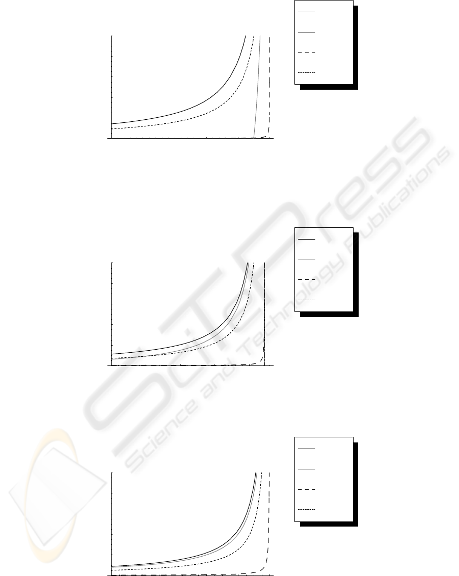
be σ = 10, 000. In Figure 1 - 3, the mean waiting
time E[W ] is depicted as the function of λ for vari-
ous µ. Note that ρ = λ
2
/σµ is the utilization of our
BMAP/M/1 queue and E[L] = λ/µ is its popula-
tion of the secure group. For the reference, not only
the bounds, but we also show the waiting time of both
the M/M/1 queue with the same utilization and the
batch-arrival M/M/1 queue where their batch size
is independent and identically to Poisson distribution
with its mean λ/µ. Comparing these graphs, although
we can see only bounds, E[W ] of the BMAP/M/1
queue is significantly larger than the ones of other
queues. Thus, we need to take into account the cor-
relation between the batches, or we underestimate the
time length of security degradation. Also, we can see
the bounds get tighter as the sojourn time of the cus-
tomer 1/µ gets shorter.
REFERENCES
Harney, H. and Muckenhirn, C. (1997a). Group key man-
agement protocol (gkmp) architecture. RFC 2094.
Harney, H. and Muckenhirn, C. (1997b). Group key man-
agement protocol (gkmp) sepcification. RFC 2093.
Kleinrock, L. (1975). Queueing Systems Vol. 1. John Wiley
and Sons.
Latouche, G. and Ramaswami, V. (1999). Introduction
to Matrix Analytic Methods in Stochastic Modeling.
SIAM.
Makimoto, N. (2001). Machigyouretsu Algorithm (Algo-
rithm of Queueing System). Asakura.
Sengupta, B. (1989). Markov processes whose steady state
distribution is matrix-exponential with an application
to the gi1 queue. Adv. Appl. Prob., (21):159–180.
Thomas, S. A. (2000). SSL and TLS Essentials: Securing
the Web. John Wiley and Sons.
Toyoizumi, H. and Takaya, M. (2004). Performance evalu-
ation of secure group communication. Journal of the
Operations Research Society of Japan, 47(1):38–50.
Tweedie, R. (1982). Operator-geometric stationary distribu-
tion for markov chains, with applications to queueing
models. Adv. Appl. Prob., (14):368–391.
Wallner, D., Harder, E., and Agee, R. (1999). Key manage-
ment for multicast: Issues and architectures. Request
for Comments: 2627.
Wolff, R. (1989). Stochastic modeling and the theory of
queues. Princeton-Hall.
Wong, C., Gouda, M., and Lam, S. (2000). Secure group
communications using key graphs. IEEE/ACM Trans.
on Networking, 8(1):16–30.
AN INFINITE PHASE-SIZE BMAP/M/1 QUEUE AND ITS APPLICATION TO SECURE GROUP COMMUNICATION
287
96 97 98 99 100
Λ
20
40
60
80
100
W
MM1
i.i.d
lower
upper
Figure 1: Upper bound and lower bound of E[W ] when µ = 1. The lines “upper ” and “lower” are the upper and lower
bounds of mean waiting time respectively. The line “i.i.d” corresponds to the batch arrival M/M/1 queue where the batch
size is independent and identically to Poisson distribution with its mean λ/µ.
314.5 315 315.5 316
Λ
20
40
60
80
100
W
MM1
i.i.d
lower
upper
Figure 2: Upper bound and lower bound of E[W ] when µ = 10.
999.2999.4999.6999.8 1000
Λ
20
40
60
80
100
W
MM1
i.i.d
lower
upper
Figure 3: Upper bound and lower bound of E[W ] when µ = 100.
SECRYPT 2006 - INTERNATIONAL CONFERENCE ON SECURITY AND CRYPTOGRAPHY
288
