Artificial Intelligence Methods Application in Liver
Diseases Classification from CT Images
Daniel Smutek
1,2
, Akinobu Shimizu
1
, Ludvik Tesar
1
, Hidefumi Kobatake
1
and
Shigeru Nawano
3
1
Tokyo University of Agriculture and Technology, Koganei, 1848588 Tokyo, Japan
2
1
st
Medical Faculty, Charles University, Prague, Czech Republic
3
National Cancer Center Hospital East, Kashiwa, 2770882 Chiba, Japan
Abstract. An application of artificial intelligence in the field of automatization
in medicine is described. A computer-aided diagnostic (CAD) system for focal
liver lesions automatic classification in CT images is being developed. The
texture analysis methods are used for the classification of hepatocellular cancer
and liver cysts. CT contrast enhanced images of 20 adult subjects with
hepatocellular carcinoma or with non-parasitic solitary liver cyst were used as
entry data. A total number of 130 spatial and second-order probabilistic texture
features were computed from the images. Ensemble of Bayes classifiers was
used for the tissue classification. Classification success rate was as high as
100% when estimated by leave-one-out method. This high success rate was
achieved with as few as one optimal descriptive feature representing the
average deviation of horizontal curvature computed from original pixel gray
levels. This promising result allows next amplification of this approach in
distinguishing more types of liver diseases from CT images and its further
integration to PACS and hospital information systems.
1 Introduction
The objective of this work is to develop a computer-aided diagnostic (CAD) system
and validate texture analysis algorithms for classification of focal hypodense hepatic
lesions.
Characterization of focal liver lesions on computed tomography (CT) depends on
correct interpretation of morphology. The aim of this study is to develop a texture
analysis concept for computer based interpretation of CT images. We concentrated on
two very common focal liver lesions: hepatocellular cancer and liver cysts.
Hepatocellular carcinoma is common throughout the world. Its incidence is higher
in cirrhotic patients. The overall survival rate ranges between 20 and 30 months, and
is influenced by the local stage of the neoplasm and by the liver function. Successful
long-term outcome is dependent on its early detection, as well as accurate delineation
of the number and location of tumor nodules.
Smutek D., Shimizu A., Tesar L., Kobatake H. and Nawano S. (2006).
Artificial Intelligence Methods Application in Liver Diseases Classification from CT Images.
In 6th International Workshop on Pattern Recognition in Information Systems, pages 146-155
DOI: 10.5220/0002444701460155
Copyright
c
 SciTePress

Computed tomography is also outstandingly suitable for detecting cystic processes
in the liver. The etiology of cysts is very wide, which means also large differences in
their clinical relevance.
Similar works of classification of liver lesions such as tumors and their
metastases, hepatic cysts, and hemangiomas, exist. They use mostly intensity-based
histogram methods [1] or second-order texture features [2;3]. Our work differs from
the previous ones by using an effective feature selection method and network
(ensemble) of Bayes classifiers which already proved their clinical usability in texture
analysis and classification of ultrasound images [4].
2 Methods
2.1 Images
Because most hepatocellular carcinoma receive equal or reduced blood supply from
both portal and arterial flow compared with surrounding noncancerous parenchyma
[5] late postcontrast enhancement images were used in our study. They were taken
approximately 3 - 5 minutes after the bolus contrast administration. The voltage of X-
ray tube was 120 kV. The resolution of the CT image was 512x512 pixels with pixel
size 0.625 mm. The slice thickness was 2 mm. Standard depth of 16 bits gray level
was used.
The images were taken from 20 adult subjects: 15 subjects with hepatocellular
carcinoma and 5 subjects with nonparasitic solitary liver cysts.
The total number of CT scans processed in this study was 535 (425 scans with
hepatocellular carcinoma and 110 scans with cysts).
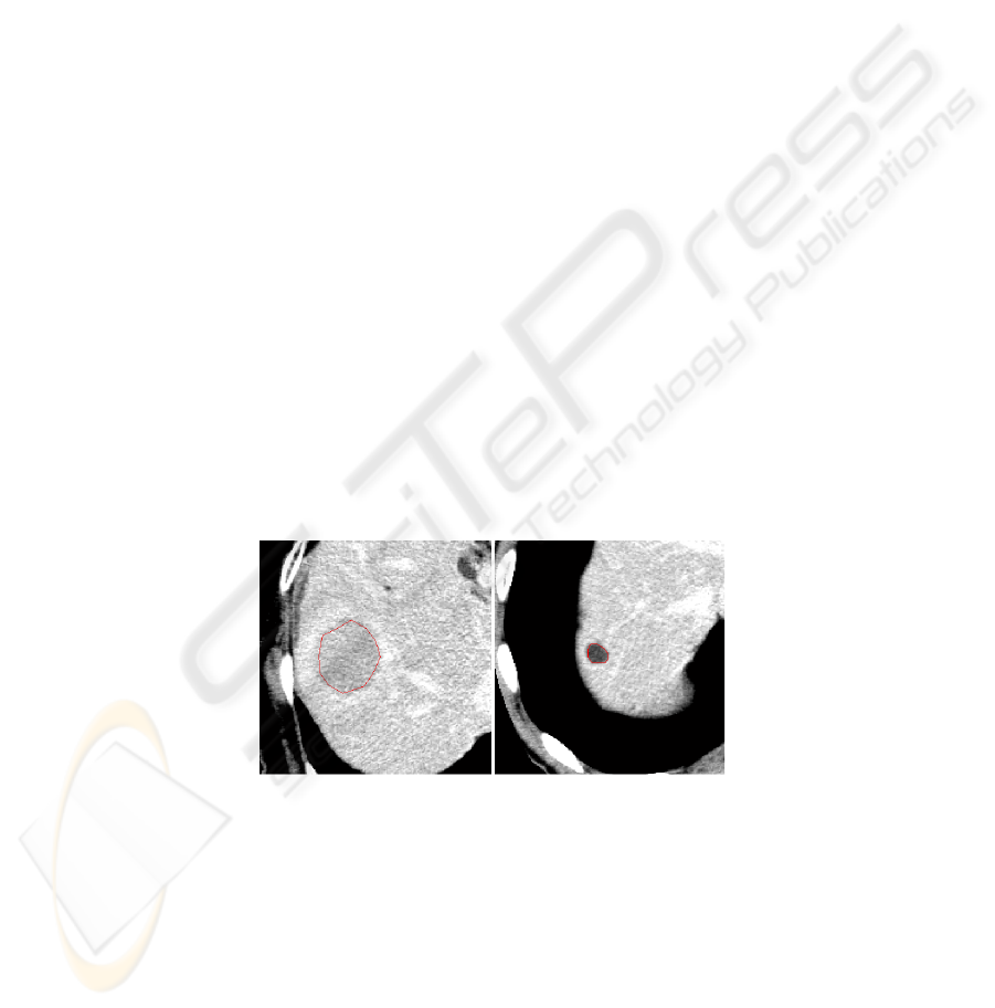
Regions of interest (ROI) with pathologic tissue (hepatocellular cancer or cyst)
were interactively defined by a physician (see Figure 1).
Fig. 1. CT images of liver with segmented boundary of hepatic lesions. On the right manually
drawn boundary (ROI) of hepatocellular cancer, on the left manually delineated cyst in liver
parenchyma.
The maximum number of non-overlapping square windows within the boundaries
was then automatically selected as the texture samples (see Figure 2). Each sample
was assigned a label according to the patient diagnosis (hepatocellular cancer, cyst).
147

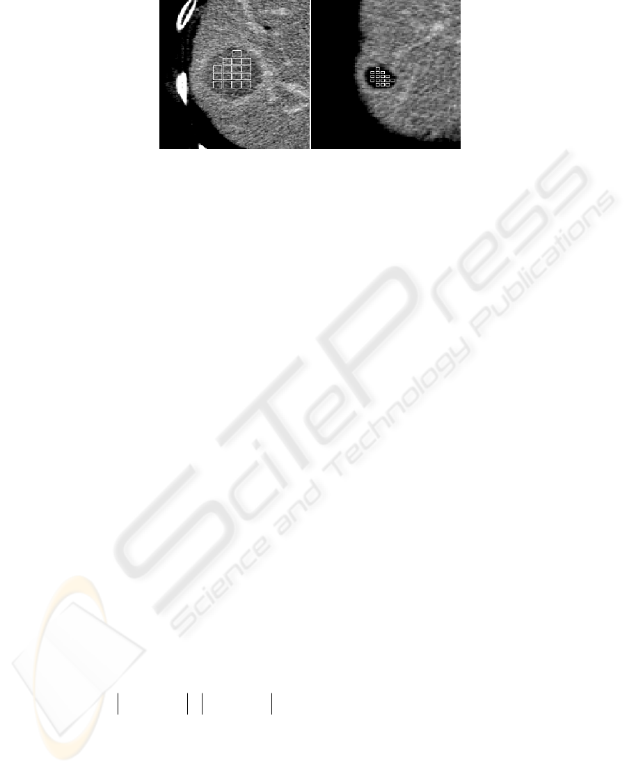
Fig. 2. CT images of liver. On the right detail of hepatocellular cancer focus with fitted texture
samples (windows of 9 x 9 pixels), on the left liver cyst with embedded texture samples with
size 7 x 7 pixels.
2.2 Texture Features
Image texture features can be computed by combining pixel gray levels in many
different ways [6]. By transforming the gray levels, it is possible to enhance some
image characteristics that are specific to a particular type of texture. Since the current
standard practice of diagnosing hepatic lesions is performed mainly subjectively,
texture characteristics observable by the human visual system are considered adequate
for an automatic computer analysis. We also note that psychophysical evidence has
shown the human visual system is capable of pre-attentive texture discrimination from
first-order to second-order properties, as defined by the moments of texture primitives
[7].
In this paper 22 first-order features were investigated: gray level of pixel (feature
called raw) and 21 spatial features based on the original gray levels of an image and
based on four different gray-level transformations [8]. In addition to first-order
features we also included second-order features in order to capture the spatial
organization of texture primitives. Therefore, most of the further 108 features used are
second-order statistical texture features based on co-occurrence matrices, which
incorporate spatial organization of texture primitives.
Spatial features
Some of the 21 spatial features are based on the original pixel gray levels p
i,j
, while
others p
m
i,j
, are based on transformations of the gray levels, where i,j denotes the
image coordinates of a pixel and m denotes a transformation. These features were
suggested by Muzzolini [8] and are summarized in this section. Four gray-level
transformations obtained from each of S samples of NxN pixels were used and are
defined as follows:
1,,,1,
)1(
,
magnitudegradient 1)
++
−+−=
jijijiji
ji
ppppp
148

jijiji
p
N
pppp
N
j
N
i
,
2
,
)2(
,
11
1
where
mean sample from difference )2
==
ΣΣ
=−=
2
curvature horizontal 3)
,1,1
,
)3(
,
jiji
jiji
pp
pp
+−
+
−=
2
curvature vertical4)
1,1,
,
)4(
,
+−
+
−=
jiji
ji
ji
pp
pp
ji
ji
pp
,
)5(
,
levelsgrey pixel original 5)
=
The Kolmogorov-Smirnov distance [9] between H
i
(p
(m)
) and )(pH
(m)
is used to
derive features f
1
,...,f
5
, from the transformations p
(m)
. The H
i
(p
(m)
) is an estimate of the
cumulative distribution function for p
(m)
computed from NxN sample i by
histogramming and
)(pH
(m)
is the robust estimate of the cumulative distribution
function mean for p
(m)
computed from H
i
(p
(m)
) over all samples i as follows:
{
}
,...,S,i)(pH LMS )(pH
(m)
i
(m)
21, == .
The LMS, Least Median of Squares, is used as a robust statistics instead of a non-
robust mean to suppress the influence of outlying values. LMS computes a value M
and a range m
T
for a data set, such that [M-m
T
; M+m
T
] is the shortest interval
containing 50% of the original data. It is a common practice to set the estimate of
standard deviation r to the value of 2.5 x 1.4826 m
T
for the case of normal errors.
Points in the range M ± r are called inliers and the remaining points are considered as
outliers. Inliers fall within 98.7% of the samples in a Gaussian distribution.
The Euclidean distance from (f
1
,...,f
5
) to their mean and median, respectively, are
used to compute features f
6
and f
7
as follows:
()()()
()()
(
)
(
)( )
()()
.5,...,2,1, feature of
median theis
ˆ
and sample, afor feature ofmean theis where
,
ˆˆ
ˆˆˆ
,
2
55
2
44
2
33
2
22
2
11
7
2
55
2
44
2
33
2
22
2
11
6
=
−+−+
−+−+−
=
−+−+
−+−+−
=
if
fff
ffff
ffffff
f
ffff
ffffff
f
i
iii
149

Features f
8
,...,f
12
are derived from the transformations p
(m)
just like features
(f
1
,...,f
5
) except that the average deviation (AD) of the pixel gray level p
(m)
i,j
is used as
the measure, where
.5,...,2,1 ,
1
)(
)(
)(
,
2
)(
=−=
ΣΣ
mpp
N
pAD
m
m
ji
ji
m
Features f
13
and f
14
are based on the Euclidean distance from (f
8
,...,f
12
) to their
mean and median, respectively. They are defined exactly the same way as the features
f
6
and f
7
with the exception that the subscripts (1,...,5) are replaced with subscripts
(8,...,12).
Features f
15
,...,f
19
are based on the transformations p
(m)
, just like features (f
1
,...,f
5
),
except that the standard deviation (SD) of the pixel gray level p
(m)
i,j
is used as the
measure, where
()
() ()
2
() () ()
,
2
() (),
1
( ) ,
1, 2,..., 5
mm
mmm
ij
ij
SD p Var p
Var p p p
N
m
=
=−
=
ΣΣ
Features f
20
and f
21
are based on the Euclidean distance from (f
15
,...,f
19
) to the mean
and median of (f
15
,...,f
19
).
Co-occurrence matrix features. Co-occurrence matrices can be used to obtain
texture features. For each NxN texture sample W taken from an image I, a set of gray
level co-occurrence matrices C
d
(i,j) is calculated for a given separation vector
d

as
follows:
(
)
⎪
⎭
⎪
⎬
⎫
⎪
⎩
⎪
⎨
⎧
=+=
∈++
−−
=
jdrIirI
Wdrrdrr
card
bNaN
jiC
d
)( and )( and
,:,
))((
1
),(









where
d

=(a,b), I(
r

) is the gray level of pixel
r

, from the interval of 0,1,…, G-1.
The image resolution of G = 64 was used, and card X is the size of the set X.
The elements of C
d
represent the frequencies of occurrence of different gray level
combinations at a distance
d

. In this paper, nine Haralick texture features [6] were
investigated.
Twelve separation vectors
d

= (1,0); (2,0); (3,0); (4,0); (1,1); (2,2); (3,3); (4,4);
(0,1); (0,2); (0,3); (0,4) were used in the experiments, resulting in twelve different
gray level co-occurrence matrices for each size of texture sample. Thus D co-
occurrence matrix features (f111-f1129) were generated for each of the sample size.
These are denoted according to the following notation: "f1dh", where d is the index of
a separation vector (of a possible twelve) and h is the number of a Haralick feature (of
a possible nine) giving D=108. For example, f195 is texture homogeneity for vector
d

=(0,1).
To achieve uniform scale, all features were normalized by their standard deviation
from zero.
150

2.3 Diagnosing
Bayes classifier [10] was selected for its best possible ability to distinguish classes
that overlap in feature space. The classifier uses the decision function
)(vd
i

over M
classes
)()|()(
iii
CpCvpvd


= , Mi ,,2,1 …
=
to assign a feature vector
v

to class
i
C
if for that vector )()( vdvd
ji


> for all
i
j
≠ , where )(
i
Cp is the a priori probability of class
i
C (i.e., the probability of
occurrence of class
i
C ) and )|(
i
Cvp

is the probability that
v

comes from
i
C (this
as the model probability function and it must be learned from a training set). A priori
probabilities of 0.5 for both classes (since hepatocellular cancer and cysts are evenly
included in our experiment) were used for estimating
)(vJ

.
The choice of model probability function
)|(
i
Cvp

is determined by discrete
quantization of the feature space.
2.4 Feature Selection Learning Method
The purpose of feature selection is to reduce the texture description from D to d
dimensions, where d<<D. Each sample of the classes (hepatocelullar carcinoma, cyst)
can be represented in terms of d features and be viewed as a vector in d-dimensional
space. From the statistical point of view, reduction of feature vector dimension is
important to determine classifier parameters reliably from a limited amount of data,
i.e., to limit the expected bias and variance of the classifier.
The goal in our approach for feature selection is to select a subset of features that
minimize the expected classification error. It is based on a direct classification error
minimization and requires a specific choice of classifier. Since the data is sufficient to
estimate probability density of a feature vector even in high dimension, Bayes
classifier is used in this approach.
We successively search for the optimal feature vector
v

of length 1
+
k by adding
a new feature in a locally optimal way to the best existing feature vector candidate of
length k. The quality
)(vJ

of a feature vector
v

(computed as above) initially
increases with increasing length of the vector and then starts to decrease due to data
over-fitting [10]. Therefore, a simple depth-first search for the optimal feature vector
cannot be used. Our algorithm therefore performs the search for optimal solutions by
a modified branch-and-bound algorithm [10].
The classifier is trained by estimating the conditional probability density for each
class by optimal histogramming. Optimal histogram resolution according to Scott’s
rule was used for the corresponding feature vector dimension and the number of
samples [11]. Our data collection mechanism produces a sufficiently large number of
samples to obtain statistically meaningful estimates this way.
151

2.5 Subject Classification
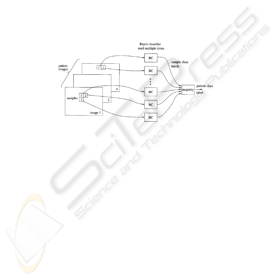
The subject classifier then works in two stages (see Figure 3): In the first stage,
individual texture samples (e.g., from 7x7 windows) from all images from a single
subject are classified independently. In the second stage the classifier outputs are
combined using majority voting to determine the class label for the given subject. The
reason for using a two-stage classifier is that the primary features exhibit a large
overlap between the classes. It is well known [12] that classifier combination can lead
to increased performance even if the individual classifiers are weak. Of the known
combination methods [13] the best performance was achieved by majority voting in
our data.
The subject is thus assigned the label C (hepatocellular cancer, cyst), which
corresponds to the class of most of its samples. For more detailed description see
Figure 3.
Fig. 3. The classifier works in two stages: In the first stage, individual texture samples from all
images of the given scan type from a single subject are classified independently using Bayes
classifier. In the second stage, the classifier outputs are combined using majority vote to
determine the class label for the given subject.
2.6 Evaluation of the Success Rate
Finally classification success rates were estimated by leave-one-out method for all
optimal feature vectors found by selection scheme Bayes classifier. Leave-one-out
means that 1. all images of one subject are removed from training set, 2. classifier is
learned on the remaining images, and 3. the images that were left out are classified
using the classifier. The three steps are repeated for all subjects. This method provides
good estimate of classifier generalization accuracy.
3 Results
For practical experiments only the faster feature selection learning method was used.
152

A total of 6,239,480 feature values (130 features for each of 47,996 samples) were
computed and the different combinations of them were used for classification. The
best value of
100)( =vJ

was achieved for several texture sample sizes and several
features.
All the features suitable for classification (which gave results with leave-one-out
error less than 0.1) and the corresponding sample sizes are shown in Table 1.
Originally, also slower Mixture model method was considered, because it should
give better results. Because even feature selection method provided right diagnosis for
every patient, we decided not to do so.
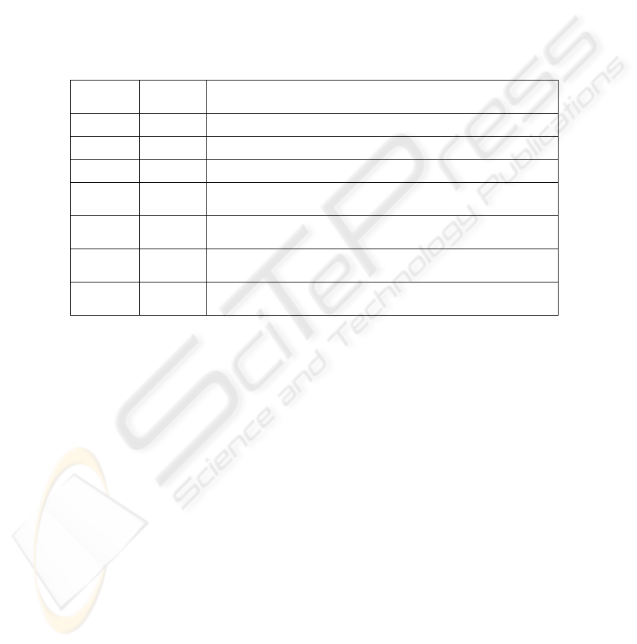
Table 1. Size of texture samples, leave-one-out classification error and the features used for the
classification.
4 Discussion and Conclusion
The results show the excellent discrimination between hepatocellular carcinoma and
liver cysts can be established on the basis as few as one optimal feature among the
130 texture characteristics tested.
From these results the principal descriptive feature can be identified: f10. Feature
f10, which was chosen among other 130 features, represents the average deviation of
horizontal curvature computed from original pixel gray levels. This feature gave
100% classification success rate in all texture samples size (from 7x7 to 19x19
pixels).
Also the most effective size of texture sample was determined. We computed
features for samples from the tiny squares of size 7x7 pixels up to large squares with
side of 41 pixels. The maximum success of 100% correct classification was achieved
for texture samples with size 9x9 to 13x13 pixels. Then with the increasing size of
side the error also increased (for 41x41 samples the total error was 0.25). The failure
of the large squares can be contributed to the fact that they do not cover the area of
ROI sufficiently and thus it results in an information wasting (a considerable big
Size of
sample
LOO
Error
Features used for classification
7x7 0.056 f10, f11, f15, f186, f2, f8, f9, raw
9x9 0 f10, f15, f20
11x11 0 f10, f129, f16, f20, f8, f9
13x13 0
f10, f11, f129, f13, f132, f157, f16, f172, f187, f2, f20,
f8, f9
15x15 0.071
f10, f11, f1117, f1127, f117, f119, f12, f127, f13, f157,
f16, f167, f172, f177, f197, f2, f20, f8, f9, raw
17x17 0.071
f10, f11, f1107, f1117, f117, f12, f13, f16, f197, f2,
f20, f8, f9, raw
19x19 0.077
f10, f11, f117, f12, f13, f147, f157, f197, f2, f20, f8, f9,
raw
153

amount of the tissue, near to the border of segmentation boundaries is not used for
computing texture features in such case).
On the other hand it can be seen that there are considerably more texture features
which are useful for successful classification in larger samples. E.g., three possible
features in 9x9 samples, six features in 11x11 samples, and thirteen texture features in
samples of 13x13 pixels. We attribute it to the fact that there is more information
about spatial organization of texture primitives available in the larger samples.
We infer that in future research the texture samples with the size 13x13 pixels and
texture feature f10 (the average deviation of horizontal curvature) will be the most
useful.
As the next step it is desirable to include more classes (diagnoses) in the
classification process. The most important which should be comprised in the very
next step are hepatic hemangiomas, focuses of liver cirrhosis and various tumor
metastases.
On the assumption that the majority of used features were higher order texture
features (and thus independent on the gray level histograms of the image but
dependent on spatial organization of texture primitives) we did not perform any image
preprocessing. Nevertheless the normalization of the images prior to computing the
texture features (e.g., by comparison with other organs in abdominal cavity or the
diaphragm) in our future experiments might get even better results.
Also the other important step, which is necessary to undertake, is to utilize all
information which is available from 3D CT images and thus using texture features
which comprise this data. The usability of non enhanced CT images and images in
earlier stages of contrast enhancement or their combination should be also explored.
Finally we can conclude that initial implementation of our CAD system is
promising for automating liver lesion classification and that it may be integrated to
Picture Archiving & Communications Systems (PACS) and to hospital information
systems.
Acknowledgements
This study was supported in part by the Grant-in-Aid for Scientific Research on
Priority Areas from Ministry of Education, Culture, Sports, Science and Technology,
Japan and in part by grant IET101050403 of Czech Academy of Sciences.
References
1. Bilello M, Gokturk SB, Desser T, Napel S, Jeffrey RB, Jr., Beaulieu CF. Automatic
detection and classification of hypodense hepatic lesions on contrast-enhanced venous-
phase CT. Med.Phys. 2004; 31: 2584-93.
2. Gletsos M, Mougiakakou SG, Matsopoulos GK, Nikita KS, Nikita AS, Kelekis D. A
computer-aided diagnostic system to characterize CT focal liver lesions: design and
optimization of a neural network classifier. IEEE Trans.Inf.Technol.Biomed. 2003; 7: 153-
62.
154

3. Klein HM, Klose KC, Eisele T, Brenner M, Ameling W, Gunther RW. [The diagnosis of
focal liver lesions by the texture analysis of dynamic computed tomograms]. Rofo 1993;
159: 10-5.
4. Smutek D, Sara R, Sucharda P, Tjahjadi T, Svec M. Image Texture Analysis of Sonograms
in Chronic Inflammations of Thyroid Gland. Ultrasound in Medicine and Biology 2003; 29:
1531-43.
5. Takayasu K, Muramatsu Y, Mizuguchi Y, Moriyama N, Ojima H. Imaging of early
hepatocellular carcinoma and adenomatous hyperplasia (dysplastic nodules) with dynamic
ct and a combination of CT and angiography: experience with resected liver specimens.
Intervirology 2004; 47: 199-208.
6. Haralick RM, Shapiro LG. Computer and Robot Vision. Reading MA : Addison-Wesley,
1992.
7. Julesz B, Gilbert EN, Shepp LA, Frish HL. Inability of humans to discriminate between
visual textures that agree in second-order statistics---revisited. Perception 1973; 2: 391-405.
8. Muzzolini R, Yang YH, Pierson R. Texture Characterization using Robust Statistics.
Pattern Recognition 1994; 27: 119-34.
9. Muzzolini R, Yang YH, Pierson R. Multiresolution Texture Segmentation with Application
to Diagnostic Ultrasound Images. IEEE Transactions on Medical Imaging 1993; 12: 108-
23.
10. Bishop CM. Neural Networks for Pattern Recognition. Oxford: University Press, 1997.
11. Scott D. Multivariate Density Estimation. New York: Wiley, 1992.
12. Rohlfing T, Pfefferbaum A, Sullivan EV, Maurer CR. Information Fusion in Biomedical
Image Analysis: Combination of Data vs. Combination of Interpretations. 2005.
13. Kittler J, Hatef M, Duin RPW, Matas J. On Combining Classifiers. IEEE Transactions on
PAMI 1998; 20: 226-39.
155