CREATING AND MANIPULATING CONTROL FLOW GRAPHS

WITH MULTILEVEL GROUPING AND CODE COVERAGE

Anastasis A. Sofokleous

Brunel University, Uxbridge, UK,

Andreas S. Andreou, Gianna Ioakim

University of Cyprus, Nicosia, Cyprus

Keywords: Control Flow Graph, Node Grouping, Code Coverage.

Abstract: Various researchers and practitioners have proposed the use of control flow graphs for investigating

software engineering aspects, such as testing, slicing, program analysis and debugging. However, the

relevant software applications support only low level languages (e.g. C, C++) and most, if not all, of the

research papers do not provide information or any facts showing the tool implementation for the control

flow graph, leaving it to the reader to imagine either that the author is using third party software for creating

the graph, or that the graph is constructed manually (by hand). In this paper, we extend our previous work

on a dedicated program analysis architecture and we describe a tool for automatic production of the control

flow graph that offers advanced capabilities, such as vertices grouping, code coverage and enhanced user

interaction.

1 INTRODUCTION

In our previous work (Andreou, Sofokleous, 2004),

we presented the design and implementation details

of a new basic program analyzer architecture. The

architecture was designed to provide the capabilities

of a program analyzer to other external applications,

such as slicing tools, test case generators, debuggers

etc. Although the result of the control flow graph

construction was accurate and clear-sighted for

small to medium programs, it became evident that

for large programs its performance and viewing-

ability were degraded. As each screen is limited by

its own resolution, then it is very obvious that the

more components a graph has, the more difficult for

a user to perceive it. In addition, layout algorithms

performance and memory requirements depend on

the number of graph elements, making it harder to

depict a graph as its size grows. The rest of the paper

is organized as follows: section 2 presents the

current research status in this area and discusses the

theoretical background of our proposition. Section 3

provides the design details of the proposed

architecture and describes its basic parts. Finally,

section 4 draws the conclusions and provides some

directions for future work.

2 LITERATURE OVERVIEW

Control Flow Graphs have been widely used in the

static analysis of software. McCabe (McCabe 1976),

was among the first that used the control flow graph

for the study of software. Furthermore, Fenton,

Whitty and Kaposi, (Fenton, Whitty et al. 1985),

studied the structuredness of software, using the

graphic representations of program flow. On the

other hand, the Program Dependence Graph (PDG)

has been proposed by Ottenstein and Ottenstein

1984 (Ottenstein, Ottenstein 1984), (Ferrante,

Ottenstein et al. 1987) addressing the internal

representation for monolithic programs (programs

that contain one unique block) and trying to

implement certain processes of software technology,

like slicing and estimation of metrics. Control flow

information indicates the possible routes of

instructions following the execution of a program

(Damian 2001). The appropriate analysis of a

259

A. Sofokleous A., S. Andreou A. and Ioakim G. (2006).

CREATING AND MANIPULATING CONTROL FLOW GRAPHS WITH MULTILEVEL GROUPING AND CODE COVERAGE.

In Proceedings of the Eighth International Conference on Enterprise Information Systems - DISI, pages 259-262

DOI: 10.5220/0002448802590262

 SciTePress

control flow graph provides information about the

run-time and non-runtime properties of programs

(e.g. determination of what functions may be called

at each application point in a program). In addition,

some other researchers have demonstrates its ability

to serve several application areas such as induction

variable elimination, type recovery etc. (Shivers

1991). Although many authors propose the use of

CFG, its extraction stays usually at a minimum

level, supporting a limited set of commands (Jones,

Mycroft 1986).

Graph visualization, is a kind of process that is

not the same for all graphs. Many characteristics

make this kind of practice different and usually

complicated. For instance, a graph of a large size

(i.e. a graph that has many elements) poses several

difficult obstacles in terms of performance and

memory. Supposing that it is feasible to layout and

display all the elements of the graph, it is still almost

impossible to distinguish the nodes from the edges

and therefore the viewing ability and usability is

dramatically decreased (Herman, Melançon et al.

2000). Therefore, reducing the number of visible

elements being viewed may turn to be very useful,

improving the clarity and the performance of the

layout and the rendering algorithms (Kimelman,

Leban et al. 1994). Such techniques are referred in

the literature as cluster analysis, grouping, clumping,

classification and unsupervised pattern recognition

(Everitt 1974), (Mirkin 1996). Many efforts have

been made thus far to develop software frameworks

intended to be used with mathematics and include

large libraries of algorithms, while others target

more general applications (Berry, Dean et al. 1999,

Cesar 1999.).

Graph architectures, like ProDAG (Richardson,

O'Malley et al. 1992), have been used as dependence

analysis tools for Ada and C++ programs. ProDAG

identifies dependencies based on the program

dependence relationships defined by Podgurski and

Clarke. Dependence analysis is performed by

ProDAG in a two-step process. First, a language-

specific intermediate representation is created, and

then language-independent analysis is performed

over this representation. In (Cooper, Harvey et al.

2002), the authors present an algorithm for building

correct control flow graphs from scheduled

assembly code. However this kind of analysis is

useful if the target code is expressed at the assembly

level.

3 EXTENDING THE BPAS

SYSTEM

The proposed Basic Program Analyzer System

(BPAS) is decomposed into two subsystems

performing two types of analysis, the runtime (or

dynamic analysis) and the non-runtime analysis (or

static analysis) respectively. Both sub-systems can

provide a mixture of information and operations

about the program under study, such as variable and

scope identification, control flow graph creation,

code coverage and running simulation. Thus,

external applications can use their functionality for

obtaining this information. While the non-runtime

analysis is carried out without executing the

program, the runtime analysis evaluates the

behaviour of the program and gathers information

during real or simulated execution. The layered

architecture is built similarly to the traditional OSI

communication standard and therefore it enjoys its

advantages as well. Each module responsible for a

specific process is placed as an intermediary layer to

the system, or as an additional layer that can be

activated at any point of time. The layered design

offers scalability and expandability to the system.

This is also supported by the present work since the

module responsible for the control flow graph

creation has been replaced with a new version

without affecting the other modules.

The most important BPAS modules are the

IOExecutive, the Parser, the Walker, the Static

Analyzer (Non-Runtime Analysis), the Dynamic

Analyzer (Runtime Analysis) and the program code

coverage. Although the BPAS works only with Java

code, its design and layered composition make

possible the use of additional programming

languages with minor adaptations in the Parser layer

and the creation of a new grammar specification.

3.1 Constructing the Control Flow

Graph with Grouping (Detail

Level)

At the stage of non-runtime program analysis, the

analyzer creates the control flow graph without

executing the program. Although the old control

flow graph algorithm proposed in (Andreou,

Sofokleous 2004) was satisfactory for small to

medium programs, it became evident that for large

programs its performance and memory requirements

were significant and its viewing ability was affected.

Having that in mind, we propose here the concept of

multi-grouping, that is, the ability to display the

ICEIS 2006 - DATABASES AND INFORMATION SYSTEMS INTEGRATION

260

same information in fewer vertices and provide the

option for the selection of the level of detail. The

basic idea is that the user defines the number of the

levels of detail before the analysis.

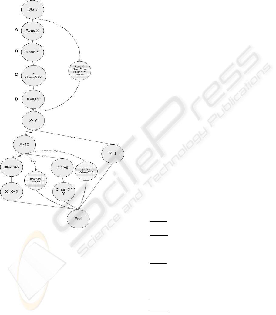
Figure 1: Multilevel Grouping.

For instance, if this level number is set to 2 the

control flow graph will have two levels of details

(figure 1). The lowest level is the default level,

which is displayed initially on screen. The default

level has 8 vertices (including Start, End nodes) and

8 edges; some of its vertices/edges belong also to the

highest level of the control flow graph (common

elements). The highest level control flow graph

having 13 vertices and 14 edges is the “expanded

graph” or the graph without grouping. Each level of

grouping has its own rules (i.e. which

statements/expressions are grouped). In the example,

the levels of detail mean that the first level will have

the grouping of neighbouring vertices that are simple

statements only. Specifically, for vertices A(Read

X), B(Read Y), C(int other=X+Y), D(X=X+Y) a new

vertex is created that has as value the value of the

A,B,C,D vertices joined with semicolons. The new

vertex ABCD is connected with a new outgoing

edge to the descendent of the D vertex and with a

new incoming edge from the precedent of the A

vertex. The new vertices and edges are displayed

with dash lines in the figure. Although the two

graphs have common edges and vertices, only edges

and vertices belonging to the selected graph net are

viewable at any point of time. The set of common

elements in this example include the vertex (X<Y)

and its outgoing edges. Having more levels involves

grouping of nested code blocks. The desired number

of levels depends on the size of the program and the

usage objective.

3.2 The Code Coverage Module

The common Code Coverage (CC) module, which is

part of the runtime analysis system, simulates the

execution of the program and at the same time it is

able to indicate the executed/covered code. Code

coverage may be used by other application systems,

such as testing systems, development tools,

debuggers etc. Such systems need to determine the

covered vertices (or the executed code/statements)

for each pair of input (test case). The particular

module is incorporated in our architecture being able

to extract not only this kind of information but

additional pieces as well, such as the executed path

from start to end, the covered code, how many times

each vertex was executed etc. The code coverage

module simulates the real execution of a program

under study (virtual running) as follows:

Step 1:

A pair of input values is given to the CC

module.

Step 2:

A control flow graph visitor takes the

values and begins the graph walking from the start

node. At each vertex, the visitor executes (simulates

the real execution of) the statements and conditions.

Step 3:

Each variable is stored in a data structure

having an initial value, a current value and a variable

name. The current variable value is updated each

time the visitor evaluates a relevant to this variable

statement.

Step 4:

The visitor marks the visited

vertices/statements.

Step 5:

The user is able to interact with the

program and view the executed vertices/statements.

In addition, information about the program or the

node is provided by the enhanced user interface.

CREATING AND MANIPULATING CONTROL FLOW GRAPHS WITH MULTILEVEL GROUPING AND CODE

COVERAGE

261

4 CONCLUSIONS AND FUTURE

WORK

This paper describes the utilization of grouping

algorithms in cooperation with control flow graphs

for software analysis purposes. While a number of

algorithms for grouping common visual graphs and

their elements have been proposed, control flow

graph clustering algorithms imply a different kind of

processing. In this context we extended our previous

work on program analysis and we replaced the

existing module that creates the control flow graph

with a new, modified algorithm that can manipulate

the control flow graph prior to displaying it so as to

provide optional levels of details. The basic program

analyzer was tested extensively in a number of

programs ranging from 100 to 20,000 lines of code,

and having different types of statements. The results

demonstrate the ability of the proposed grouping

feature of the new control flow algorithm is able to

handle large programs with different types of

statements (or equivalently different complexity). In

addition, this paper introduces a new software

module, which performs code coverage processing,

the latter enhancing and completing the proposed

architecture.

With the above feature the modified Basic

Program Analyzer broadens its scope and allows its

usage by additional types of application tools: The

grouping of vertices in different levels of detail

provides the means to investigate larger programs,

since performance and memory no longer constrain

the process. In addition, the ability to select the level

of display detail aids the easy comprehension of a

large program graph, since the analyzer is able to

depict the same information with less graph

elements.

REFERENCES

Andreou, A. and Sofokleous, A., 2004. Designing and

implementing a layered architecture for dynamic and

interactive program analysis, Proceedings of IADIS

International Conference, Portugal, Spain.

Berry, J., Dean, N., Goldberg, M., Shannon, G. and

Skiena, S., 1999. Graph Drawing and Manipulation

with LINK, Proceedings of the Symposium on Graph

Drawing GD’97, Springer–Verlag pp425-437.

Cesar, C., L., 1999, 1999.-last update, graph foundation

classes for java, IBM2005.

Cooper, K., D., Harvey, T., J. and Waterman, T., 2002.

Building a Control-flow Graph from Scheduled

Assembly Code. TR02-399.

Damian, D., 2001. On Static and Dynamic Control-Flow

Information in Program Analysis and Transformation,

Ph.D. Thesis, BRICS Ph.D. School, University of

Aarhus, Aarhus, Denmark

Everitt, B., 1974. Cluster Analysis. 1st edn. Heinemann

Educational Books.

Fenton, N., E., Whitty, R., W. and Kaposi, A., A., 1985. A

generalised mathematical theory of structured

programming. Theoretical Computer Science, 36, pp.

145-171.

Ferrante, J., Ottenstein, K., J. and Warren, J., D., 1987.

The program dependence graph and its use in

optimization. ACM Transactions on Programming

Languages and Systems, 9(3), pp. 319-349.

Herman, I., Melancon, G. and Marshall, M.S., 2000.

Graph Visualization and Navigation in Information

Visualization: a Survey. IEEE Transactions on

Visualization and Computer Graphics, 6, pp. 1-21.

Jones, N., D. and Mycroft, A., 1986. Data flow analysis of

applicative programs using minimal function graphs,

Proceedings of the 13th ACM SIGACT-SIGPLAN

symposium on Principles of programming languages,

St. Petersburg Beach, Florida, pp296-306.

Kimelman, D., Leban, B., Roth, T. and Zernik, D., 1994.

Reduction of Visual Complexity in Dynamic Graphs,

Proceedings of the Symposium on Graph Drawing GD

’93, Springer–Verlag.

MCcabe, T., 1976. A Complexity Measure. IEEE

Transactions on Software Engineering, SE-2, no.4, pp.

308-320.

Mirkin, B., 1996. Mathematical Classification and

Clustering, Kluwer Academic Publishers.

Ottenstein, K., J. and Ottenstein, L., M., 1984. The

program dependence graph in a software development

environment. Proceedings of the ACM

SIGSOFT/SIGPLAN Software Engineering

Symposium on Practical Software Development

Environments, 19(5), pp. 177-184.

Richardson, D., J., O'Malley, T., O., Moore, C., T. and

AHA, S., L., 1992. Developing and Integrating

ProDAG in the Arcadia Environment, In SIGSOFT

'92: Proceedings of the Fifth Symposium on Software

Development Environments, pp109-119.

Shivers, O., 1991. Control-Flow Analysis of Higher-Order

Languages. CMU-CS-91-145. Carnegie Mellon

University, Pittsburgh, Pennsylvania

ICEIS 2006 - DATABASES AND INFORMATION SYSTEMS INTEGRATION

262