A LOAD BALANCING SCHEDULING APPROACH FOR

DEDICATED MACHINE CONSTRAINT

Arthur M. D. Shr, Alan Liu

Department of Electrical Engineering, National Chung Cheng University, Chia-Yi 621, Taiwan, R.O.C.

Peter P. Chen

Department of Computer Science, 298 Coates Hall, LSU, Baton Rouge, LA 70803, USA

Keywords: Load Balancing Scheduling, Dedicated Machine Constraint, Least Slack, Resource Schedule and Execution

Matrix, Semiconductor Manufacturing.

Abstract: The constraint of having a dedicated machine for photolithography process in semiconductor manufacturing

is one of the new challenges introduced in photolithography machinery due to natural bias. With this

constraint, the wafers passing through each photolithography process have to be processed on the same

machine. The purpose of the limitation is to prevent the impact of natural bias. However, many scheduling

polices or modeling methods proposed by previous research for the semiconductor manufacturing

production have not discussed the dedicated machine constraint. In this paper, we propose the Load

Balancing (LB) scheduling approach based on a Resource Schedule and Execution Matrix (RSEM) to tackle

this constraint. The LB scheduling approach is to schedule each wafer lot at the first photolithography stage

to a suitable machine according to the load balancing factors among machines. We describe the algorithm of

the proposed LB scheduling approach and RSEM in the paper. We also present an example to demonstrate

our approach and the result of the simulations to validate our approach.

1 INTRODUCTION

Semiconductor manufacturing systems are different

from the traditional manufacturing systems, such as

a flow-shops manufacturing system in assembly

lines or a job-shops manufacturing system. In a

semiconductor factory, one wafer lot passes through

hundreds of operations, and the processing

procedure takes a few months to complete. The

operations of semiconductor manufacturing

incrementally develop an IC product layer by layer.

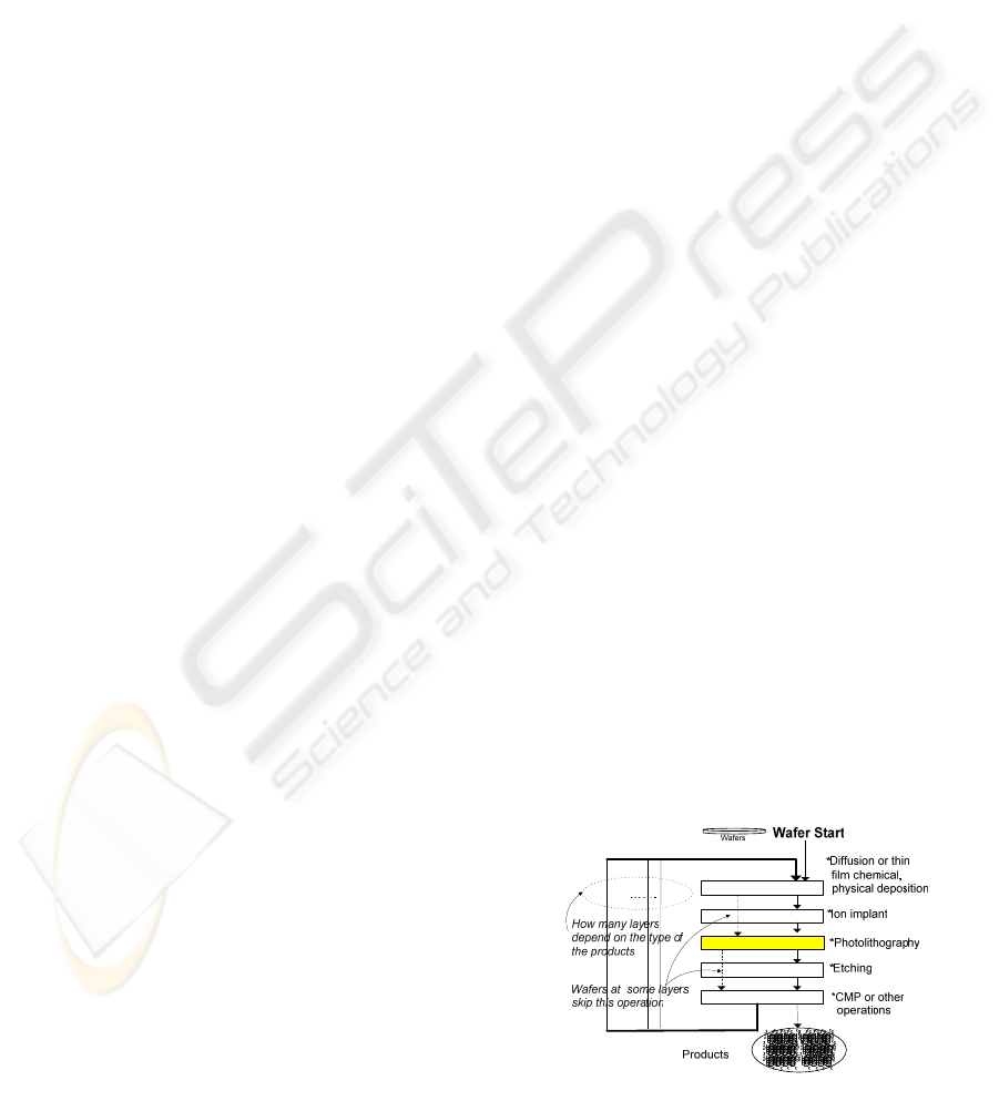
Figure 1 shows the concept of the process flow of a

semiconductor manufacturing system, a re-entrant

production line (Kumar, 1993) (Kumar, 1994).

One of the challenges in the semiconductor

manufacturing systems is the dedicated

photolithography machine constraint which is

caused by the natural bias of the photolithography

machine. Natural bias will impact the alignment of

patterns between different layers. The smaller the

dimension of the IC products (wafers), the more

difficult they will be to align between different

layers. The wafer lots passing through each

photolithography stage have to be processed on the

same machine. The purpose of the limitation is to

prevent the impact of natural bias and to keep a good

yield of the IC product. Figure 2 describes the

dedicated machine constraint. When wafer lots enter

each photolithography operation stage, with this

constraint, the wafer lots dedicated to machine X,

they need to wait for machine X, even if there is no

wafer lot waiting for machine Y, which is idle. On

the other hand, when wafer lots enter into other

Figure 1: The process flow of semiconductor

manufacturing, a re-entrant line.

170

M. D. Shr A., Liu A. and P. Chen P. (2006).

A LOAD BALANCING SCHEDULING APPROACH FOR DEDICATED MACHINE CONSTRAINT.

In Proceedings of the Eighth International Conference on Enterprise Information Systems - AIDSS, pages 170-175

DOI: 10.5220/0002454801700175

 SciTePress

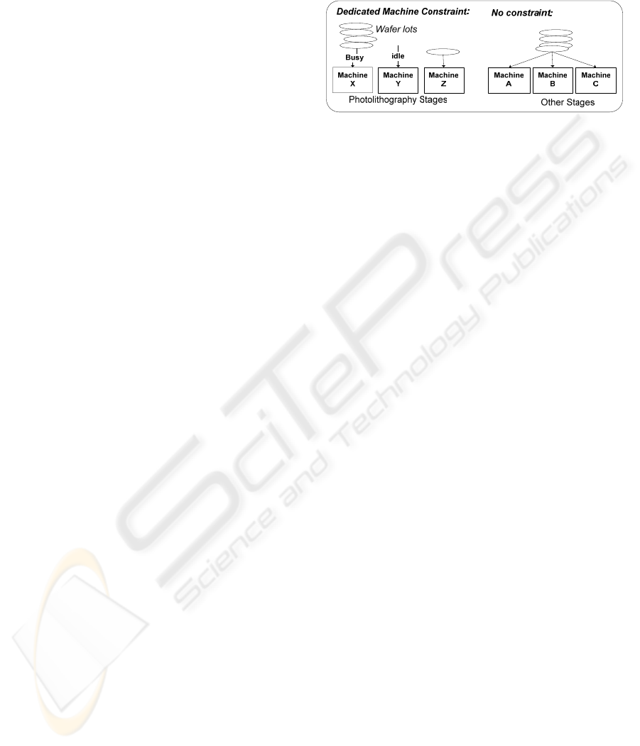
operation stages, without any machine constraints,

the wafer lots can be scheduled to any machine of A,

B or C as long as they become idle.

The constraint is the most important challenge to

improve productivity and fulfill the request for

customers as well as the main contributor to the

complexity and uncertainty of semiconductor

manufacturing. If we randomly schedule the wafer

lots to arbitrary photolithography machines at the

first photolithography stage, then the load of all

photolithography machines might become

unbalanced. This load balancing issue derived

mainly from the dedicated photolithography

machine constraint. This happens because once the

wafer lots have been scheduled to one of the

machines at the first photolithography stage, they

must be assigned to the same machine in the

subsequent photolithography stages until they have

passed the last photolithography stage. Therefore,

the short time of unexpected breakdown of one

machine will cause a pile up of many wafer lots

waiting for the machine and the situation makes the

machine critical to the factory.

Therefore, the unbalanced load among

photolithography machines will mean that some of

the photolithography machines will become idle and

remain so for a while, due to the fact that no wafer

lots can be processed, and the other will always be

busy while many wafer lots in the buffer limited to

this machine are awaiting processing. As a result,

the performance of the factory will have been

decreased and impacted. The wafer lots of a load

unbalancing factory usually need to be switched

from the highly congested machines to the idle

machines. It relies on experienced engineers to

manually handle alignment problem of the wafer lots

with a different situation off-line. It is inefficient to

determine one lot at a time which wafer lot and

machine need be switched. Moreover, this method

cannot meet the fast-changing market of the

semiconductor industry.

Motivated by the issues described above, we

propose a Load Balancing (LB) scheduling approach

based on a Resource Schedule and Execution Matrix

(RSEM) to tackle the dedicated machine constraint.

By selecting a wafer lot which has the maximum

waiting step and a wafer lot which has the smallest

load, the LB method could schedule each wafer lot

at first and unconstrained photolithography stage to

a suitable photolithography machine.

The paper is organized as follows: we describe

the related research in Section 2. Section 3 depicts

the algorithm of the proposed LB scheduling

approach. An example of semiconductor factory

applying LB scheduling approach is described in

Section 4. Section 5 shows the simulation results

that validated our approach. Section 6 discuses the

conclusion.

Figure 2: Dedicated machine constraint and load balancing

2 RELATED RESEARCH

By using a queuing network model, a “Re-Entrant

Lines” model has been proposed to provide the

analysis and design of the semiconductor

manufacturing system. (Kumar, 1993) (Kumar,

1994). These scheduling policies have been

proposed to deal with the buffer competing problem

in the re-entrant production line, wherein they pick

up the next wafer lot in the queue buffers when

machines are becoming idle. Wein’s research used a

Brownian queuing network model to approximate a

multi-class queuing network model with dynamic

control to the process in the semiconductor factory

(Wein, 1998). A special family-based scheduling

rule, Stepper Dispatch Algorithm (SDA-F), is

proposed to the wafer fabrication system (Chern and

Liu, 2003). SDA-F uses a rule-based algorithm with

threshold control and least slack principles to

dispatch wafer lots in photolithography stages. A

stochastic dynamic programming model proposed

for scheduling new wafer lot release and bottleneck

processing by stage in the semiconductor factory

(Shen and Leachman, 2003). This scheduling policy

incorporates analysis of uncertainties in products'

yield and demand.

Dynamic Scheduling System is a dynamic

artificial intelligent scheduling approach that focuses

on the most urgent unsolved problem (Hildum,

1994). Another research uses the Petri Net approach

to modeling, analysis, simulation, scheduling and

the control of the semiconductor manufacturing

system (Zhou and Jeng, 1998). Two researches

developed simulations to model the

photolithography process, one of them proposed a

Neural Network approach to develop an intelligent

scheduling method according to a qualifying matrix

and the lot scheduling criteria to improve the

performance of the photolithography machines

(Arisha and Young 2004). The other one is to decide

A LOAD BALANCING SCHEDULING APPROACH FOR DEDICATED MACHINE CONSTRAINT

171

the wafer lots assignment of the photolithography

machines at the time when the wafer lots were

released to manufacturing system to improve the

load-balancing problem (Mönch, et al. 2001).

3 RESOURCE SCHEDULE AND

EXECUTION MATRIX (RSEM)

The RSEM method consists of three modules Task

Generation, Resource Calculation, and Resource

Allocation modules. The first module is to model the

tasks for the scheduling system. For example, in the

semiconductor factory, the tasks are the procedures

of processing wafer lots, starting from the raw

material until the completion of the IC products. We

generate a two-dimension matrix for the tasks that

are going be processed by machines. One dimension

is reserved for the tasks t

, t

,…, t

, the other is to

represent the periodical time event (or step) s

,…,s

. Each task has a sequential pattern to

represent the resources it needed during the process

sequence from a raw material to a product. We

define each type resource as r

, r

, …, r

, where it

means a particular task needs the resources in the

sequence of r

and r

following that until r

is gained.

Therefore, the matrix looks as follows:

. . . . . s

. . s

.. .. .. r

. .. .. .. ..

.. .. r

.. .. .. .. ..

. .. ..

.. .. r

. . .

.. .. r

.. .. ..

The symbol, r

in the Matrix[t

, s

] is to represent

the fact that the task t

needs of the resource

(machine) r

at the time s

. If t

starts to be processed

at s

and the total step numbers of t

is p, we will fill

its pattern into the matrix from Matrix[t

, s

] to [t

j+p-1

]. All the tasks, t

,…t

, follow the illustration

above to form a task matrix in the task generation

module. To represent the dedicated machine

constraint in the matrix for this research, the symbol

, a replacement of r

, is to represent that t

has

been dedicated to number x of type k machine at s

The symbol w

is to represent the wait situation

when the machine r

cannot serve t

at s

. We will

insert this symbol in the Resource Allocation

module later.

The Resource Calculation module is to

summarize the value of each dimension as the

factors for the scheduling rules of the Resource

Allocation module. For example, we can acquire

how many steps t

needed to be processed by

counting task pattern of t

dimension in the matrix.

We can also realize how many wait steps t

has had

by counting w

from start step to current step of t

dimension in the matrix. Furthermore, if we count

the r

in s

dimension, we can know how many tasks

will need the machine m

of resource r

at s

Before we can start the execution of the

Resource Allocation module, we need to generate

the task matrix, obtain all the factors for the

scheduling rules, and build up the rules. The module

is to schedule the tasks to the suitable resource

according to the factors and predefined rules. To

represent the situation of waiting for r

; i.e., when t

can not take the resource of r

at the time s

, then we

will not only insert w

in the pattern of t

, but also

need to shift the following pattern to the next step in

the matrix. Therefore, we can obtain the updated

factor for how many tasks wait for r

at s

only if we

have counted w

by the dimension s

. We can also

obtain the factor for how many wait step that t

has

had only if we have counted w

, 1

≤

o by t

dimension in the matrix

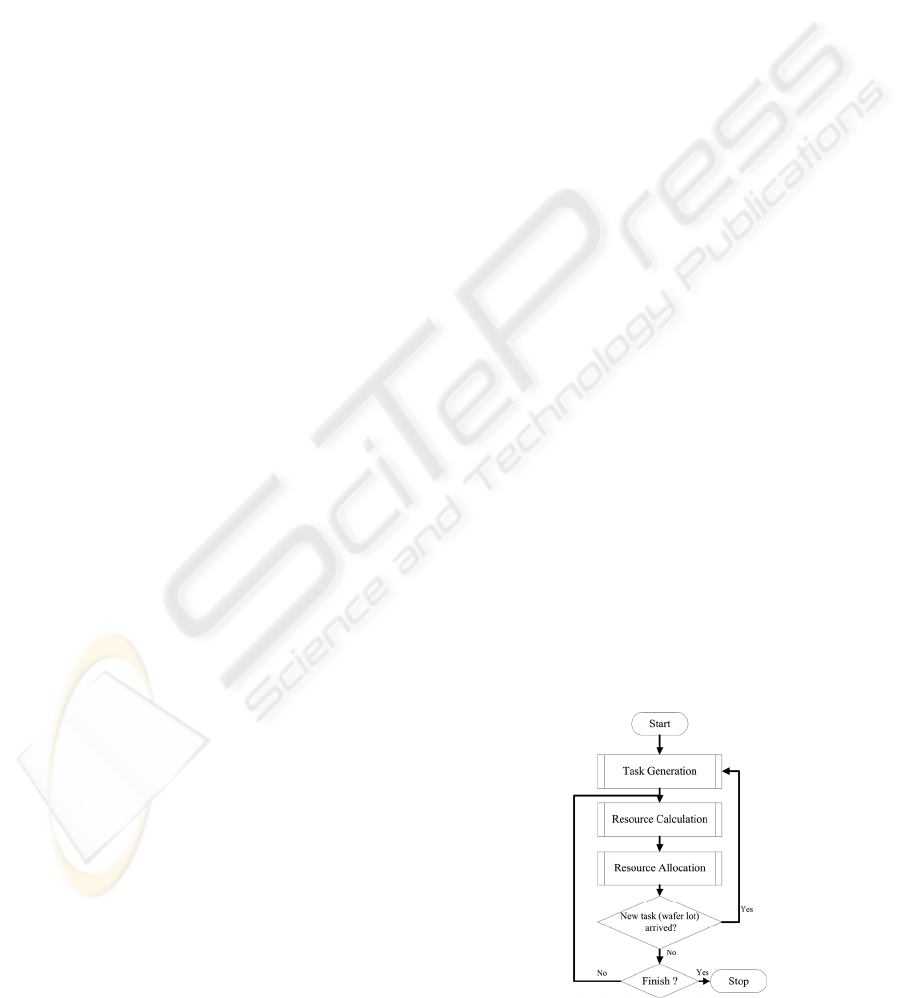
To better understand our proposed scheduling

process, the flowchart of RSEM is shown in Figure

3. The process of using the RSEM starts from the

Task Generation module and it will copy the

predefined task patterns of tasks into the matrix.

Entering the Resource Calculation module, the

factors for the tasks and resources will be brought

out at the current step. This module will update these

factors again at each scheduling step. The execution

of scheduling process is in the Resource Allocation

module. When we have done the schedule for all the

tasks for the current step, we will return to check for

new tasks and repeat the whole process again by

following the flowchart. We will exit the scheduling

process when we reaches the final step of the last

task if there is still no new task appended to the

matrix. After that, the scheduling process will restart

immediately when the new tasks arriving in the

system.

Figure 3: Scheduling flowchart.

ICEIS 2006 - ARTIFICIAL INTELLIGENCE AND DECISION SUPPORT SYSTEMS

172

4 LOAD BALANCING

SCHEDULING APPROACH

After obtaining the process flow for customer

product from the database of semiconductor

manufacturing, we can use a simple program to

transform the process flow into our matrix

representation. There exist thousands of wafer lots

and hundreds of process steps in a typical factory.

We start from transforming the process pattern of

wafer lots into a task matrix. We let r

represent the

photolithography machine and r to represent non-

photolithography machines. The symbol r

in the

Matrix[i,j] is to represent the wafer lot t

need of the

photolithography machine m

at the time s

with

dedicated machine constraint, while r

≠

2) is to

represent the wafer lot t

need of the machine type k

and the machine m

at s

j’

≠

j’) without dedicated

machine constraint. There is no assigned machine

number for the photolithography machine before the

wafer lot has passed first photolithography stage.

Suppose that the required resource pattern of t

is as

follows: r

, and

starts the process in the factory at s

. We will fill its

pattern into the matrix from Matrix[t

] to

Matrix[t

], which indicates that the total number

of the steps for t

is 25. The following matrix shows

the pattern of t

. The wafer lot t

in the matrix has

the

same required resource pattern as t

but starting at s

The wafer lot t

in the matrix starts from s

, and then

it requires the same type resource, the

photolithography machine, but does not have the

same (number) machine at s

. This represents that t

needs the machine m

, while t

has not been

dedicated to any machine yet. Moreover, two tasks,

and t

might compete with the same resource r

if the resource of r

is not enough for them at s

The definitions and formulae of these factors for

the LB scheduling approach in the Resource

Calculation module are as follows:

W: wafer lots in process,

P: numbers of photolithography machines,

K: types of machine (resource)

(1) Required resource (machine):

(1.1) How many wafer lots will need the photolithography

machine m

at s

(with dedicated machine constraint):

PxrstMatrixsrRR

jij

≤≤=

∑

∈

1 ,],[),(

(1.2) How many wafer lots will need the other k type

machine at s

(without dedicated machine constraint):

KkkrstMatrixsrRR

jijk

1 ,2,],[),( ≤≤≠=

∑

∈

(2) Count step:

(2.1) How many wait steps the t

has had before s

KkwstMatrixtWaitStep

stepcurrent

startj

kjii

≤≤

∑

1 ,],[)(

(2.2) How many steps t

will have.

∑

≠=

stepend

startj

jii

stMatrixtSteps

""],[)(

(3) The load factor of machine m

, wafer lots

remanding

photolithography stages

∑

∈Wt

xiiijx

mtpmtRtsmLoad })(|)(*{),(

(3.1) How many remaining photolithography stages for t

PxrstMatrixtR

stepend

currentj

jii

≤≤

∑

1 ,],[)(

(3.2) pm(t

): dedicated photolithography machine number

of t

Load is defined as the wafer lots limited to

machine m multiple their remaining layers of

photolithography stage. Load is a relative parameter,

representing the load of the machine and wafer lots

limited to one machine compared to other machines.

The larger load factor means that the more required

service from wafer lots has been limited to this

machine.

The LB scheduling approach uses these factors

to schedule the wafer lot to a suitable machine at the

first photolithography stage which is the only

photolithography stage without the dedicated

constraint. Suppose we are currently at s

, and the

LB scheduling system will start from

photolithography machine. We check if there is any

wafer lot which is waiting for the photolithography

machines at the first photolithography stage. LB will

assign the m

with smallest Load(m

, s

) for them one

by one. After that, these wafer lots have been

dedicated a photolithography machine. For each m

LB will select one of the wafer lots dedicated to m

which has the largest WaitStep(t

) for it. Load(m

, s

)

of m

will be updated after these two processes. The

other wafer lots dedicated to each m

which can not

be allocated to the m

at current step s

will insert a

for them in their pattern. For example, at the step

, t

has been assigned to m

, therefore, t

i+1

will

have a w

being inserted into at s

, and then all the

following required resource of t

i+1

will shift one

step.

.. .. s

.. s

.. .. .. .. .. .. .. .. .. .. .. .. .. .. .. ..

.. ..

A LOAD BALANCING SCHEDULING APPROACH FOR DEDICATED MACHINE CONSTRAINT

173

The following matrix shows the situation. All the

other types of machine will have same process

without need of being concerned with the dedicated

machine constraint. Therefore, we assigned one of

the wafer lots which has the largest WaitStep(t

then the second largest one, and so on for each

machine r

. LB will insert a w

for the wafer lots do

not be assigned to machines r

at current step.

Therefore, WaitStep(t

) is to represent the delay

status of t

.. .. s

.. s

.. ..

i+1’

.. .. .. ..

↑ → →

→ →

We assume that all the resource types for the

wafer lots will have the same process time in this

example, i.e., all the steps have the same time

duration. The assumption simplifies the real

semiconductor manufacturing system and helps us

focus on the issue of the dedicated machine

constraint. In fact, it is not difficult to approach the

real cases on a smaller scale time step. Another issue

is that the machines in the factory have capacity

limitation due to the capital invention, which is the

resource constraint. How to make the most profit for

the invention mostly depends on optimal resource

allocation techniques. However, most scheduling

polices or methods can provide neither the exact

allocation in accepted time, nor a robust and

systematic resource allocation strategy. We use the

RSEM to represent complex tasks and allocate

resources by the simple matrix calculation. This

reduces much of the computation time for the

complex problem.

Our LB scheduling system provides two kinds of

functions. One is that we can follow the predefined

rules from expert knowledge to obtain the resource

allocation result at each step quickly by the factors

summarized from task matrix. The other is that we

could predict the bottleneck or critical situation

quickly by executing proper steps forward. This can

also evaluate the predefined rules to obtain better

scheduling rules for the system at the same time.

5 SIMULATION RESULT

We have done two types of simulations for a Least

Slack (LS) time scheduling policy and our LB

scheduling method. The LS time scheduling has

been developed in the research, Fluctuation

Smoothing Policy for Mean Cycle Time (FSMCT)

(Kumar and Kumar, 2001) in which the FSMCT is

for re-entrant production lines. The entire class of

LS policies has been proven stable in a deterministic

setting (Lu and Kumar, 1991, and Kumar, 1994).

The LS scheduling policy sets the highest priority to

a wafer lot whose slack time is the smallest in the

queue buffer of one machine. When the machine is

going to idle, it will select the highest priority wafer

lot in the queue buffer to service next. However, the

simulation result shows that our proposed LB is

better than the LS method. For simplifying the

simulation to easily represent the scheduling

methods, we have made the following assumptions:

(1) Each wafer lot has the same process steps and

quantity.

(2) All photolithography and other stages have the same

process time.

(3) There is no breakdown event in the simulations.

(4) There is unlimited capacity for non-photolithography

machines.

The simulations are to use two photolithography

machines and 200 wafer lots. Each wafer lot in the

first simulation has 28 steps, and 5 of them are

photolithography stages. While each wafer lot in the

second simulation has 40 steps and 9 of them are

photolithography stages. In the following two

simulation patterns, r represents the non-

photolithography stage; and r

the photolithography

stage. The wafer lot t

starts to process in the factory

when t

has passed two steps (s

). t

starts when t

has passed three steps (s

) . We simulate the wafer

arrival rate between two wafer lots as a Poisson

distribution.

Simulation I: tasks matrix

,…………………………………………………………..s

:rrr

rrrrr

rrrrrrrrr

rrrrrr

rrr

: rrr

rrrrr

rrrrrrrrr

rrrrrr

rrr

: rrr

rrrrr

rrrrrrrrr

rrrrrr

rrr

200

: :

Simulation II: tasks matrix

,……………………………………………………………s

:rrr

rrrrr

rrrrrrrrr

rrrrrr

rrr

: rrr

rrrrr

rrrrrrrrr

rrrrrr

rrr

: rrr

rrrrr

rrrrrrrrr

rrrrrr

rrr

200

: :

We applied the LS and LB method for these two

photolithography machines to select the next wafer

lot to process in the simulations. When the wafer lot

needs to wait for its dedicated machine, we insert a

“w” in the process pattern of the wafer lot to

represent the situation. After completing the

simulations, we count the pattern of wafer lots to

obtain how much time they have used. The

simulation result is shown in Figure 4.

ICEIS 2006 - ARTIFICIAL INTELLIGENCE AND DECISION SUPPORT SYSTEMS

174

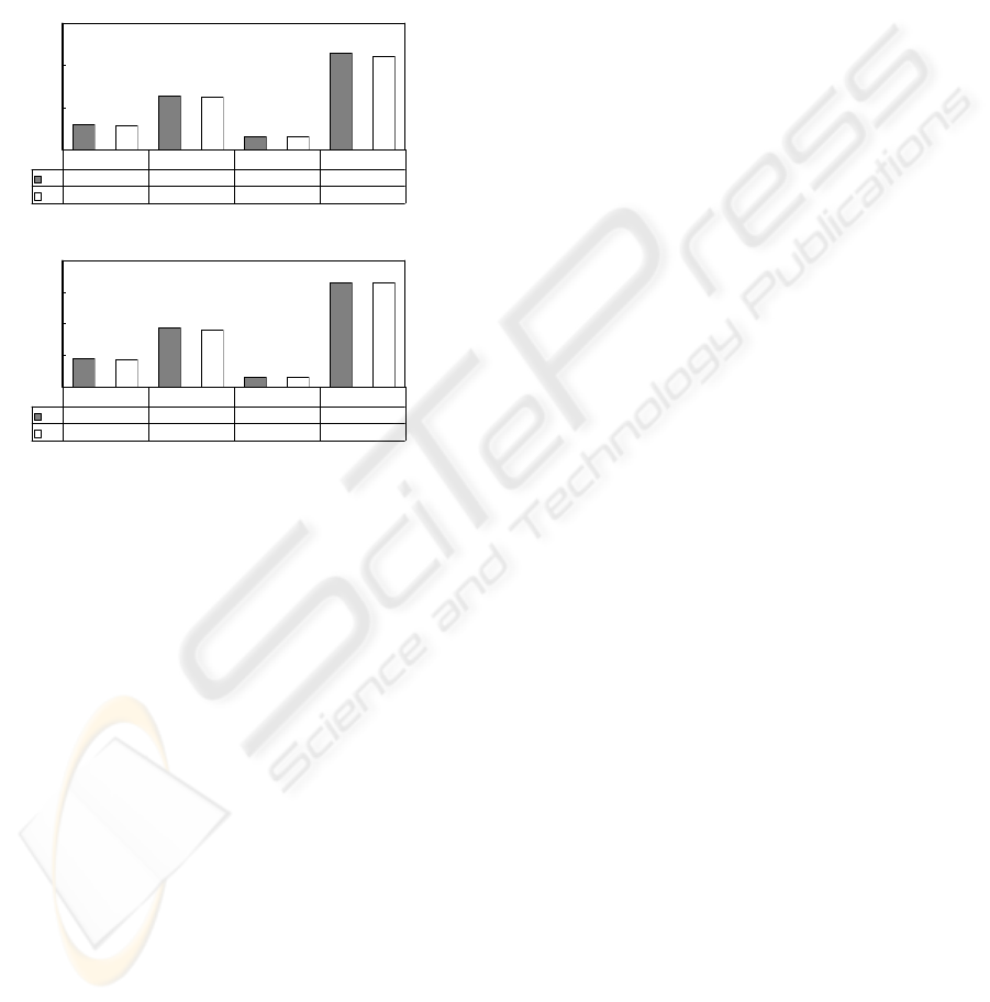
Comparing the mean of cycle time, the LS

method has an average 128.52 steps in simulation I

and 371.64 steps in simulation II. The LB method

has an average 125.63 and 356.50 steps in

simulation I and II. LB is better than LS 2.30% in

simulation I and 4.25% in simulation II. For the

deviation of steps of all wafer lots in these two

simulations, the LB approach is better than the LS

approach.

Simulation I

228

56.62

125.63

222

58.50

128.52

100

200

300

58.50 128.52 30 228

56.62 125.63 30 222

σ Mean Min Max

Simulation II

178.73

661

356.50

656

371.64

173.30

200

400

600

800

178.73 371.64 59 661

173.30 356.50 59 656

σ Mean Min Max

Figure 4: Result of simulation I & II.

Although the simulations are simplified, they

reflect the real situation we have met in the factory.

It is not difficult to extend the simulation with more

machines, wafer lots, and stages. We can use

different numbers of r

together, e.g., r

, r

, or

,…, for the task patterns to represent different

process time of different photolithography stages.

6 CONCLUSION

To provide the solution to the issue of dedicated

machine constraint, the proposed Load Balancing

(LB) scheduling approach has been presented. Along

with providing the LB scheduling approach to the

dedicated machine constraint, we also presented a

novel model--the representation and manipulation

method for the task patterns. The simulations also

showed that our proposed LB scheduling approach

was better than the LS method. The advantage of LB

is that we could easily schedule the wafer lots by

simple calculation on a two-dimensional matrix.

Moreover, the matrix architecture is easy for

practicing other semiconductor manufacturing

problems in the area with a similar constraint.

ACKNOWLEDGEMENTS

This research was supported in part by the Ministry

of Education under grant EX-91-E-FA06-4-4 and

the National Science Council under grant NSC-94-

2213-E-194-010 and NSC-92-2917-I-194-005. This

research was also partially supported by the U.S.

National Science Foundation grant No. IIS-0326387.

One of us, A. Shr, is grateful to Ms. Victoria Tangi

for English proof-reading.

REFERENCE

Arisha, A. and Young, P., 2004 Intelligent Simulation-

based Lot Scheduling of Photolithography Toolsets in

a Wafer Fabrication Facility. 2004 Winter Simulation

Conference, pp. 1935-1942.

Chern, C. and Liu, Y., 2003. Family-Based Scheduling

Rules of a Sequence-Dependent Wafer Fabrication

System. In IEEE Transactions on Semiconductor

Manufacturing, Vol. 16, No. 1, pp. 15-25.

Hildum, D., 1994. Flexibility in a Knowledge-based

System for Solving Dynamic Resource-Constrained

Scheduling Problem. Umass CMPSCI Technical

Report UM-CS-1994-77, University of Massachusetts,

Amherst.

Kumar, P.R., 1993. Re-entrant Lines. In Queuing Systems:

Theory and Applications, Special Issue on Queuing

Networks, Vol. 13, Nos. 1-3, pp. 87-110.

Kumar, P.R., 1994. Scheduling Manufacturing Systems of

Re-Entrant Lines. Stochastic Modeling and Analysis of

Manufacturing Systems, David D. Yao (ed.), Springer-

Verlag, New York, pp. 325-360.

Kumar, S. and Kumar, P.R., 2001. Queuing Network

Models in the Design and Analysis of Semiconductor

Wafer Fabs. In IEEE Transactions on Robotics and

Automation, Vol. 17, No. 5, pp. 548-561.

Lu, S.H. and Kumar, P.R., 1991. Distributed Scheduling

Based on Due Dates and Buffer Priorities. In IEEE

Transactions on Automatic Control, Vol. 36, No. 12,

pp. 1406-1416.

Mönch, L., et al., 2001. Simulation-Based Solution of

Load-Balancing Problems in the Photolithography

Area of a Semiconductor Wafer Fabrication Facility.

2001 Winter Simulation Conference, pp. 1170-1177.

Shen, Y. and Leachman, R.C., 2003. Stochastic Wafer

Fabrication Scheduling. In IEEE Transactions on

Semiconductor Manufacturing, Vol. 16, No. 1, pp. 2-

14 .

Wein, L.M., 1998. Scheduling Semiconductor Wafer

Fabrication. In IEEE Transactions on Semiconductor

Manufacturing, Vol. 1, No. 3, pp. 115-130.

Zhou, M. and Jeng, M.D., 1998. Modeling, Analysis,

Simulation, Scheduling, and Control of Semiconductor

Manufacturing System: A Petri Net Approach. In

IEEE Transactions on Semiconductor Manufacturing,

Vol. 11, No. 3, pp. 333-357.

A LOAD BALANCING SCHEDULING APPROACH FOR DEDICATED MACHINE CONSTRAINT

175