
Prediction of Protein Tertiary Structure Class from
Synchrotron Radiation Circular Dichroism Spectra
Andreas Procopiou
1
, Nigel M. Allinson
1
, Gareth R. Jones
2
, David T. Clarke
2
1
Department of Electrical and Electronic Engineering, The University of Sheffield,
Mappin Street, Sheffield, UK
2
CCLRC Daresbury Laboratory, Warrington, UK,
Abstract. A new approach to predict the tertiary structure class of proteins from
synchrotron radiation circular dichroism (SRCD) spectra is presented. A
protein’s SRCD spectrum is first approximated using a Radial Basis Function
Network (RBFN) and the resulting set is used to train different varieties of
Support Vector Machine (SVM). The performance of three well known multi-
class SVM schemes are evaluated and a method presented that takes into
account the properties of spectra for each of the structure classes.
1 Introduction
Synchrotron radiation circular dichroism (SRCD) [1] spectroscopy provides a simple
and relatively fast experimental procedure for revealing the secondary structure of
proteins and their folding motifs. It can be exploited for almost any size of
macromolecule and can even assist in the determination of some elements of a
protein’s tertiary structure. Proteins are classified into five main structural groups
according to their domains: α, β, α + β, α/β and unordered or denatured proteins that
have little ordered structure [2]. The circular dichroism (CD) spectra of proteins
exhibit unique characteristics depending on these five classes [3]. The CD spectra of
α proteins exhibit strong double minima at 222 nm and 208 – 210 nm as well as a
stronger maximum at 192 – 194 nm. The β proteins produce spectra that usually have
a single negative and a single positive band; however the positions of these bands
vary and their intensities are much lower than those of α proteins. For α + β and α/ β
proteins, the intensities of spectra are more similar to the alpha helix structure since
usually it dominates over those of beta sheets. The CD spectra of other proteins have
a strong negative band between 198 – 200 nm.
The first attempt to relate CD spectra to the tertiary structure involved the visual
examination of the spectra together with several other criteria for determining the
class [4]. A mathematical technique of cluster analysis was proposed in [5], and was
able to identify α, α/β proteins but performed very poorly when tested on
polypeptides which were wholly α-helical or β-sheet, identifying them both as
belonging to the α/ β class.
Procopiou A., M. Allinson N., R. Jones G. and T. Clarke D. (2006).
Prediction of Protein Tertiary Structure Class from Synchrotron Radiation Circular Dichroism Spectra.
In 6th International Workshop on Pattern Recognition in Information Systems, pages 58-67
DOI: 10.5220/0002478200580067
Copyright
c
SciTePress

In this paper we use a Radial Basis Function Network (RBFN) and various Support
Vector Machines (SVM) to classify proteins into the five classes according to their
SRCD spectra. When an SRCD spectrum is presented to the system, the RBF network
provides a set of basis functions that are used as inputs to an SVM, which decides the
class of the test protein. The SVM was chosen as they have several attractive
characteristics as they are statistically-based models rather than loose analogies of
natural learning systems, and they have some theoretical guarantee of performance
[6]. They are designed for two-class problems as they seek to find a hyperplane in the
feature space that maximally separates the two target classes.
The remainder of the discussion is organized as follows – the task is placed in its
context by providing some background on the structural organization of proteins,
outlining both RBF networks and SVMs, and then details of the experimental
procedures. This is followed by a discussion of the results when different varieties of
SVM are used.
2 Protein Structure
All structural and functional properties of the proteins derive from the chemical
properties of their polypeptide chains. There are four levels of protein structural
organization: primary, secondary, tertiary and quaternary.
The primary structure of a protein is the sequence of amino acids from which it is
constructed [7]. The secondary structure refers to the arrangement of the amino acids
that are close together in a chain. There are three common secondary structures in
proteins, namely alpha helices, beta sheets and turns [2]. Those that cannot be
cataloged as one of these standard three classes are usually grouped into a category
called other. A beta sheet is constructed from beta strands form different regions of
the polypeptide chain; in contrast to an alpha helix, which is formed from one
continuous region. Thus beta sheets are composed of two or more straight chains that
are hydrogen-bonded side by side. If the amino termini are at the same end, the sheet
is termed parallel, and if the chains run in the opposite directions (amino termini at
opposite ends), the sheet is termed antiparallel. Turns are the third of the three main
secondary structures with approximately one-third of all residues in globular proteins
contained in turns that reverse the direction of the polypeptide chain.
Tertiary structure refers to the complete three-dimensional structure of the
polypeptide units of a given protein. Included in this description is the spatial
relationship of different secondary structures to one another within a polypeptide
chain and how these secondary structures themselves fold into the three-dimensional
form of the protein. For small globular proteins of 150 residues or fewer the folded
structure involves a spherical compact molecule composed of secondary structural
motifs with little irregular structure. For larger proteins the tertiary structure may be
organized around more than one structural unit, each of these called a domain.
However those interactions are fewer than the interactions of the secondary structural
elements within a domain [2].
Finally the highest level of proteins structural organization is the quaternary
structure. It results from the association of independent tertiary units through surface
interaction to form a functional protein.
59

The two main classification schemes that categorize proteins according to their
structure are the Structural Classification of Proteins (SCOP) [8] and the CATH [9].
The SCOP system currently shows 1028 unique folds although CATH shows 709. In
the SCOP proteins are classified into five main structural classes: α structures where
the core is build up mainly from alpha helices; β structure which comprise mainly
beta sheets; α+β structures, where proteins have alpha helices and beta sheets often in
separated domains, and α/β structures, where proteins have intermixed segments that
often alternate along the polypeptide chain. The fifth class refers to unordered or
denatured proteins that have little ordered structure. In the CATH the classes α+β and
α/β are combined to one class, the rest of them are the same.
3 Introduction to Employed Pattern Recognition Methods
3.1 Radial Basis Function Network
The Radial Basis Function Network is a widely used fast learning algorithm, first
introduced by Broomhead and Lowe [10]. RBF networks can perform both
classification and function approximation. For classification, the attraction of RBFs
can be explained by Cover’s theorem on the separability of patterns. This theorem
states that nonlinearly separable patterns can be separated linearly if the pattern is cast
nonlinearly into a higher dimensional space. Concerning function approximation,
theoretical results on multivariate approximation constitute the basic justifying
framework. In this paper, RBFs are only introduced as a technique for function
approximation.
The essential form of the RBF neural networks mapping is given by:
y
k
= w
ki
ϕ
i
(x)
i=1
M
∑
+ b
(1)
where w are the weight parameters and
ϕ
is the basis function [11]. There are several
forms of basis function with the most common being the Gaussian:
ϕ
i
(x) = e
−
x −
μ
i
2
2
σ
i
2
(2)
where x is the n-dimensional input vector with elements
x
i
and
μ
i
is the vector
determining the centre of the basis function.
Training Radial Basis Function Network
Four parameters are adjusted during training. Namely, the number of basis functions
M, the width parameters,
σ
, the centre locations,
μ
and the weights, w
i
. The optimal
number of centers, M, for a given set is found by using a series of trial values and
computing the corresponding prediction error which is estimated using various model
selection criteria such as generalized cross validation (GCV)[12, 13]. The number
60

with the minimum prediction error is chosen as the optimal i.e. the estimated
prediction error is the smallest.
The location of the centers can be found in a variety of ways. The simplest is to
choose the centers as a subset of the data points. The choice can be random or linearly
spread along the data set. Unsupervised techniques can be used to cluster the input
vector and then using the centers of the clusters as the centers of the basis functions.
The most common algorithm used is the well-known K-means algorithm. The width
parameter is usually chosen to be the same for all basis functions and its value to be
some multiple of the average spacing between the basis functions. This ensures that
the basis functions are overlapping to some degree and hence give a relatively smooth
representation of the distribution of the training data.
Given the width and the centers of the basis functions, the weights
w
i
can be
calculated. As derived in [12] the weights are found using:
w = A
−1
H
T
y
(3)
where H is an N x M matrix such that
H
nm
=
ϕ
m
(x
n
) , and is called the design
matrix.
A
−1
, the variance matrix, is given by A
−1
= H
T
H +Λ
⎛
⎝
⎜
⎞
⎠
⎟
−1
. The elements of
the matrix Λ are all zero except for the regularization parameters along its diagonal.
3.2 Support Vector Machines
Support Vector Machine is one kind of learning machines based on statistical learning
theory. It was firstly introduced by Vapnik [14]. This paper only considers the use of
SVMs for pattern classification, although they have also been applied to other areas
such as regression and novelty detection. The basic idea of applying an SVM to
pattern classification can be stated briefly as following: First, map the input vectors
into one feature space (possible at a higher dimension), either linearly or nonlinearly,
which is relevant with the selection of the kernel function. Then, within the feature
space from the first step, seek an optimized linear division, i.e., construct a
hyperplane that separates the two classes (this can be extended to multi-class). SVM
training always seeks a global optimized solution and avoids overfitting, so it has the
ability to deal with a large number of features.
For a two-class classification problem consider the data set x of N samples
< x
1
, y
1
>,...,< x
N
, y
N
> . Each sample is composed of a training example
x
i
of length
k, with elements
x
i
=< x
1
, x
2
,..., x
k
> , and target value y
i
∈{−1, 1} . The decision
function implemented by the SVM can be written as:
f (x) = s ign
α
i
i=1
N
∑
y
i
K(x
i
, x) + b
⎛
⎝
⎜
⎜
⎞
⎠
⎟
⎟
(4)
61

Where the coefficients
α
i
are the Lagrange multipliers and are obtained by solving
the following convex Quadratic Programming (QP) problem [6]:
Maximize
α
i
i=1
N
∑
−
1
2
α
i
α
j
y
i
y
j
j =1
N
∑
i=1
N
∑
K(x
i
, x
j
)
(5)
Subject to
0 ≤
α
i
≤ C
α
i
1=1
N
∑
y
i
= 0
(6)
The coefficients
α
i
are equal to zero for all the training samples, expect the support
vectors (i.e. the samples that lies on the hyperplane). In the above formulation the
regularization parameter, C, is a constant determining the trade-off between two
conflicting goals, maximizing of the margin and minimizing the misclassification
error.
The kernel,
K(x
i
, x
j
) , computes the inner product in feature space as a direct
operation upon the data samples in their original space [15]. If the feature-space is of
much higher dimension than the input space, this implicit calculation of the dot-
product removes the need to explicitly perform calculation in feature space.
Consequently, if an effective kernel is used, finding the separating hyperplane can be
done without any significant increase in computation time. Typical kernel functions
are:
K(x
i
, x
j
) = (x
i
⋅ x
j
)
d
(7)
K(x
i
, x
j
) = e
− x
i
−x
j
2
σ
2
(8)
Equation (7) is the polynomial kernel function of degree d, which will revert to a
linear function when d is set to one. Equation (8) is a Gaussian kernel with a single
parameter σ.
For a given dataset, only the kernel function and the regularization parameter C are
selected to specify a SVM. The latter is varied through a wide range of values and the
optimal value is found using cross-validation. The choice of kernel and its parameters
is important since if they are poorly chosen the hypothesis modeling the data can be
oversimplify or too complex leading to poor generalization. The best way to make
the appropriate choice is using cross-validation since the choice is validated by
numerous independent tests. However a large data set is required for this method.
Various methods for estimating the kernel parameter, based on theoretical arguments
without the use of additional validation data have been proposed, with the most
economical approach is to use the leave-one-out cross validation procedure [6].
62

Multi-class SVM
SVM are inherently binary classifiers so techniques are needed to extend the method
to handle multiple classes. The goal of such techniques is to map the generalization of
the binary classifiers to a multi-class domain.
One vs. One Classifier
The One vs. One classifier system was proposed by Friedman [16] and has become
the most popular and successful multi-class SVM method. This classifier creates a
binary SVM for each combination of classes possible. Then for each unseen example,
each binary SVM assigns one vote to one of the two competitive classes and the
example is assigned to the class with the higher overall votes.
DAGSVM
DAGSVM stands for Directed Acyclic Graph SVM. This method was proposed by
Platt [17]. It employs exactly the same training phase as in “One vs. One” method
described above. However it characterizes itself in the classification phase by
constructing a rooted tree structure. Each node on the tree is a binary SVM for a pair
of classes. At the lowest level the number of leaves corresponds to the number of
classes. Every non-leaf node has two edges one that corresponds to not being the first
class and the other corresponds to not being the second class.
One Vs Rest Classifier
This method requires the building of many binary SVMs as the number of different
classes. Each attempts to construct a decision boundary separating one class from the
rest. Creating the models is accomplished by assigning the label “+1” to one class and
the label, “-1”, to all remaining classes.
The advantage of this method is that there are few SVMs involved, resulting in
much faster evaluation than the previous schemes. However, since all classes are
involved in each SVM, training of the SVMs can be time-consuming.
4 Method for Predicting the Protein Tertiary Structure Class
The reference set consisted from 28 proteins, as shown in the Table 1. According to
the SCOP system, eight of them belong to class α, five to class β, six to class α+β
five to class α/β and four to class “others”. Each CD spectrum has wavelength range
of 168 – 260 nm with values been recorded every 0.5 nm.
RBFs were used to approximate each spectrum as described above. The input data
were the wavelength values, which of course is the same for all spectra. The target
values were the intensity values for each of the spectra. The form of basis function
used was the Gaussian as it is the most commonly used function. Since the input data
are linearly spread from 168 to 260 at steps of 0.5, then there is no requirement to use
any algorithm to determine the location of the centers. Instead the centers are linearly
spread across the above range at constant steps depending on the number of centers.
The width parameter was chosen to be the same for all basis functions. Its value was
63

set to be equal to the spacing between the basis functions. Finally the optimal value
for the number of centers, M, had to be found. For this, the generalized cross
validation (GCV) was used. The GCV was calculated from three centers up to and
including 40 centers, keeping all other parameters the same. The graph of M against
the GCV value is shown in Fig 1.
Table 1. Protein refernce set.
Name Code Name Class
Chymotrypsin
CHYM
β
Cytochrome C CYTC
α
Elastase
ELAS
β
Haemoglobin HAEM
α
Lactate
Dehydrogenase
LADH
/
αβ
T4 lysozyme
LYSO
αβ
+
Myoglobin MYOG
α
Papain
PAPN
αβ
+
Ribonuclease
RIBO
αβ
+
Flavodoxin
FLAV
/
αβ
Glyceraldehyde-3-
phosphate
dehydrogenase
GPDH
/
αβ
Prealbumin
PREA
β
Subtilisin BPN
SUBN
/
αβ
Ttriosephosphate
isomerase
TPIS
/
αβ
R1 from E. coli
ECOR
/
αβ
Poly-glu PGAC
α
Poly-glu (random) PGAR other
Hen lysozyme
LYSM
αβ
+
Thermolysin
THML
αβ
+
Poly-glu (random) PGAS other
Poly-glu (random) PGAL other
Polylysine (random) PLYS other
Concanavalin a
CNCA
β
Beta-LG
BLAC
β
Human Serum Albumin HSA
α
Calmodulin CALMOD
α
Melittin MELI
α
Tropomyosin TROPO
α
64
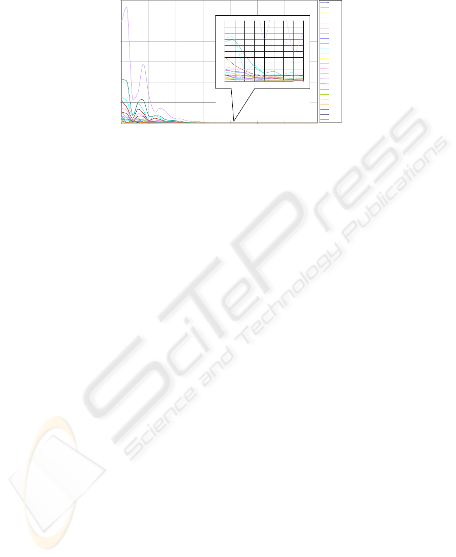
GCV
20
40
60
80
100
120
Number of centers
0
3 8 13 18 23 28 33 38
0
0.01
0.02
0.03
0.04
0.05
0.06
0.07
0.08
0.09
0.1
21 22 23 24 25 26 27 28 29
CHYM
CYTC
ELAS
HAEM
LADH
LYSO
MYOG
PAPN
RIBO
FLAV
GPDH
PREA
SUBN
TPIS
ECOR
PGAC
PGA
R
LYSM
THML
PGAS
PGAL
PLYS
CNC
A
BLAC
Fig. 1. Graph of GCV as function number of RBF centers for all proteins.
The graph shows that most M values have a minimum value at about 25. Thus this
value was chosen for all spectra. Having chosen all parameters the RBF network was
trained for each of the spectra. The regularization parameter λ was estimated for each
of the spectra. The output of the network was the weights, w, which is a vector with
25 values.
The new input space, W, is a matrix combining the weights of all the spectra and is
used to train different multi-class SVMs. The first approach uses the “One vs. One”
method, the second one is the “One vs. Rest”, and the third is the DAGSVM. Finally
the last method takes into account the properties of the spectra for each of the classes.
For each method the optimum kernel and the corresponding parameters values are
found using the Leave-One-Out cross validation process. This procedure consists of
removing from the training data one element, constructing the decision rule on the
basis for the remaining elements and then testing on the removed element. This
method produced an almost unbiased estimator [18].
To apply the “One vs. One” method, ten binary classifiers have to be constructed.
The optimal kernel was found to be the RBF function with the width parameter set to
0.0031 and the regularization parameter C set to 100. However, the results were not
very satisfactory as only 60% of the proteins are classified correctly.
The DAGSVM requires the same number of binary classifiers; however it
produced much better results. For this method, again the kernel was chosen to be the
RBF function but with the width parameter set to 0.05 and C set to 100. The results
show that 80% of all proteins were correctly classified. In addition, all of the β and
“others” proteins are correctly classified.
Applying the “One vs. Rest” multi-class scheme to the data produced even better
results and only five binary classifiers are needed. The optimum kernel was found to
be again the RBF function with the width parameter set to 0.0016 and C set to 100.
Only three of the proteins where misclassified (90% correctly classified). As in the
DAGSVM method, all the proteins that belong to either β or “others” class were
correctly classified.
In the last method, the combined properties of the CD spectra were taken into
account. As mentioned at the introduction the three classes α, α + β, α/β have similar
spectra, thus one binary classifier was employed to distinguish them from “others”
proteins and the β proteins. A second classifier was used to distinguish β proteins,
65
from the “others” proteins. The third classifier was employed to separate the proteins
belonging in class α/β. Thus the last one is used to separate the classes α and α + β
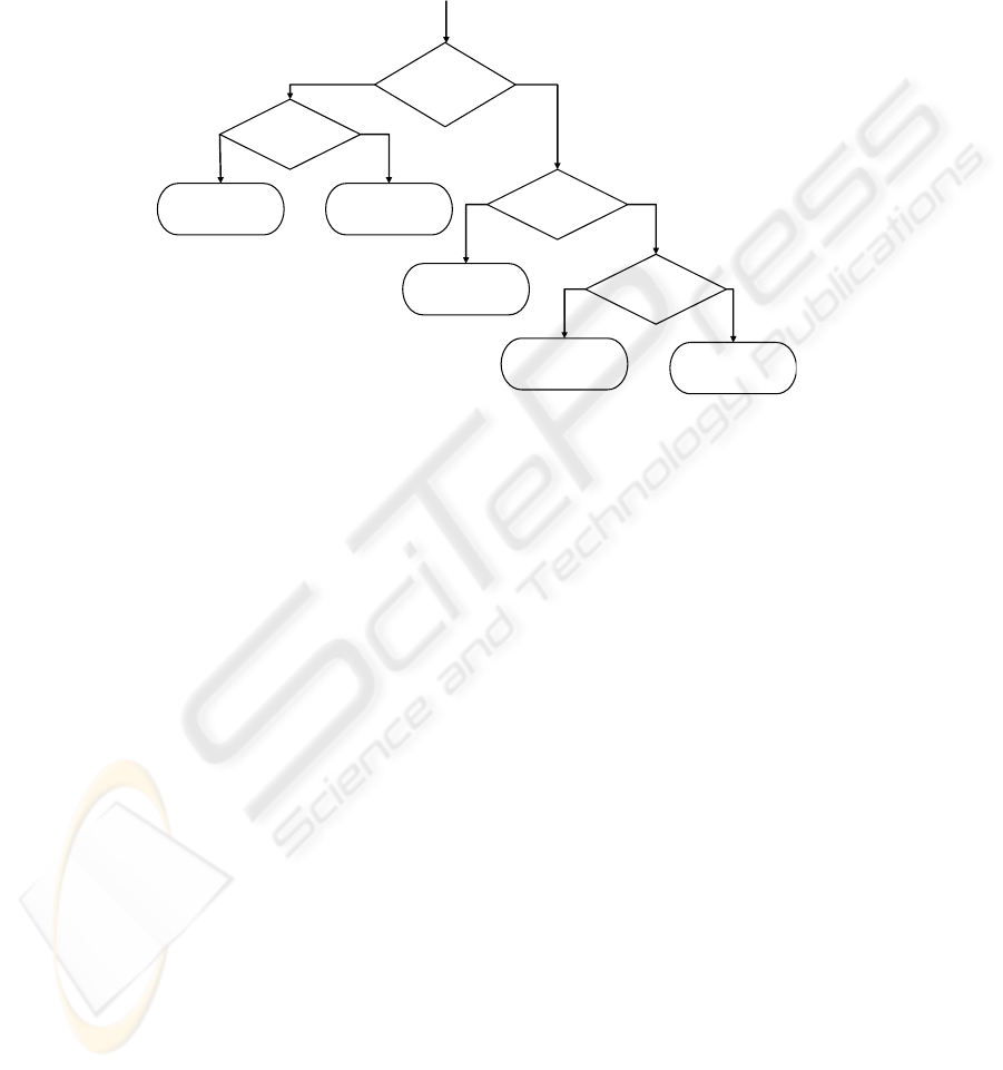
Thus this method only uses four binary classifiers. Fig. 4 summaries the above
procedure.
Fig. 2. Flow chart for classifying proteins using SRCD spectra.
The two first SVM binary classifiers are linear with C set to 1. The third one is a
non-linear classifier. The kernel function was chosen to be a Gaussian function and
the optimal width parameter was found to be 0.1 and C is again set to 100. The last
classifier is also non-linear but with the kernel function chosen to be polynomial in
the power of 11.
This method produced the best results with only two proteins misclassified. The
first one is the T4 lysozyme (LYSO), which is α + β protein but it is classified as α
protein. This is due to the fact that although the T4 lysozyme is very helical at 67%,
there are some β-sheets (10%). This protein is classified as α protein in the CATH
database, thus it is marginal. In addition there is no other similar protein in the
training set. The system was also unable to classify the Cytochrome C (CYTC), which
is α protein. The protein falls on the hyperplane separating the classes α and α + β.
This is due to its relatively small value of alpha helix fraction and also again there is
not a similar protein in the set.
5 Conclusion
This paper presents a new approach to predict the tertiary structure class of proteins
from synchrotron radiation circular dichroism (SRCD) spectra. The three most
commonly used multi-class SVM schemes were employed. Good results were
achieved using the “One vs. Rest” method where only three proteins where
misclassified. However the results were improved further when we take into account
Is it in class
“others” or
b
eta?
Is it in class
β?
Test protein belongs
to class “others”.
Test protein belongs
to class β.
Test protein
Is it in class
α/β?
Is it in class
α+β or in α?
Test protein belongs
to class α/β.
Test protein belongs
to class α+β.
Test protein belongs
to class α.
66

the properties of the spectra in each class. With this method only four binary
classifiers were employed and only two proteins where misclassified. In addition the
system was able to classify correctly all of the proteins belong to either β, or α/β or
“others” class. The experimental determination of additional protein CD spectra is in
progress. This will, hopefully, provide a more balanced training set and so enable
more accurate prediction of protein structures.
References
1. Wallace, B.A. and R.W. Janes, Synchrotron radiation circular dichroism spectroscopy of
proteins: secondary structure, fold recognition and structural genomics. Current Opinion in
Chemical Biology, 2001. 5(5): p. 567-571.
2. Whitford, D., Proteins : structure and function. 2005, Chichester, West Sussex, England ;
Hoboken, NJ: John Wiley & Sons c2005.
3. Fasman Gerald, D., Circular dichroism and the conformational analysis of biomolecules.
1996, New York ; London: Plenum Press.
4. Manavalan, P. and W.C. Johnson, Sensitivity of Circular-Dichroism to Protein Tertiary
Structure Class. Nature, 1983. 305(5937): p. 831-832.
5. Venyaminov, S.Y. and K.S. Vassilenko, Determination of Protein Tertiary Structure Class
from Circular Dichroism Spectra. Analytical Biochemistry, 1994. 222(1): p. 176.
6. Scholkopf, B. and A.J. Smola, Learning with kernels : support vector machines,
regularization, optimization, and beyond. Adaptive computation and machine learning.
2002, Cambridge, MA ; London: MIT Press.
7. Branden, C. and J. Tooze, Introduction to protein structure. 1999, New York: Garland
c1999.
8. Murzin, A.G., et al., SCOP: A Structural Classification of Proteins Database for the
Investigation of Sequences and Structures. Journal of Molecular Biology, 1995. 247(4): p.
536.
9. Pearl, F., et al., The CATH Domain Structure Database and related resources Gene3D and
DHS provide comprehensive domain family information for genome analysis. Nucleic
Acids Research, 2005. 33(Supp): p. D247-D251.
10. Broomhead, D.S. and D. Lowe, Multi-Variable Function Interpolation and Adaptive
network. Complex System, 1988: p. 2:321.
11. Bishop, C.M., Neural networks for pattern recognition. 1995, Oxford: Clarendon Press
c1995.
12. Orr, M.J.L., Introduction to Radial Basis Function Networks. 1996, University of
Edinburgh: Edinburgh, Scotland, UK.
13. Orr, M.J.L. Optimising the Widths of RBFs Radial Basis Functions. in Fifth Brazilian
Symposium on Neural Networks. 1998. Belo Horizonte, Brazil.
14. Vapnik, V., The nature of statistical learning theory. 1995, New York ; London: Springer.
15. Shawe-Taylor, J. and N. Cristianini, Kernel methods for pattern analysis. 2004, Cambridge,
UK ; New York: Cambridge University Press.
16. Friedman, J., Another approach to polychotomous classification. Technical report Stanford
University, UA, 1996.
17. Platt, N.C.J. and J. Shawe-Taylor, Large magin dags for multiclass classification. Technical
report, Microsoft Research, Redmond, US, 1999.
18. Chapelle, O., et al., Choosing Multiple Parameters for Support Vector Machines. Machine
Learning, 2001. 46(1/3): p. 131-160.
67
