
Large Scale Face Recognition with Kernel Correlation
Feature Analysis with Support Vector Machines
Jingu Heo, Marios Savvides and B. V. K. Vijayakumar
Department of Electrical and Computer Engineering
Carnegie Mellon University, U.S.A
Abstract. Recently, Direct Linear Discriminant Analysis (LDA) and Gram-
Schmidt LDA methods have been proposed for face recognition. By utilizing the
smallest eigenvalues in the within-class scatter matrix they exhibit better
performance compared to Eigenfaces and Fisherfaces. However, these linear
subspace methods may not discriminate faces well due to large nonlinear
distortions in the face images. Redundant class dependence feature analysis
(CFA) method exhibits superior performance compared to other methods by
representing nonlinear features well. We show that with a proper choice of
nonlinear features in the CFA, the performance is significantly improved.
Evaluation is performed with PCA, KPCA, KDA, and KCFA using different
distance measures on a large scale database from the Face Recognition Grand
Challenge (FRGC). By incorporating the SVM for a new distance measure, the
performance gain is significant regardless of which algorithm is used for feature
extraction, with our proposed KCFA+SVM performing the best at 85% at 0.1%
FAR where the baseline PCA gives only 12% at 0.1% FAR.
1 Introduction
Machine recognition of human faces from still and video images is an active research
area due to the increasing demand for authentication in commercial and law
enforcement applications. Despite some practical successes, face recognition is still a
highly challenging task due to large nonlinear distortions caused by normalization
errors, expressions, poses and illumination changes. Two well-known algorithms for
face recognition are Eigenfaces 1 and Fisherfaces 2. The Eigenfaces method
generates features that capture the holistic nature of faces through the Principal
Component Analysis (PCA), which determines a lower-dimensional subspace that
offers minimum mean squared error approximation to the original high-dimensional
data. Instead of seeking a subspace that is efficient for representation, the Linear
Discriminant Analysis (LDA) method seeks directions that are efficient for
discrimination. Due to the fact that the number of training images is smaller than the
number of pixels, the within-class scatter matrix S
w
is singular causing problems for
LDA. The Fisherfaces performs PCA to overcome this singular-matrix problem and
applies LDA in the lower-dimensional subspace. Recently, it has been suggested that
the null space of the S
w
is important for discrimination. The claim is that applying
PCA in Fisherfaces may discard discriminative information since the null space of the
S
w
contains the most discriminative power. Fueled by this finding, Direct LDA
Heo J., Savvides M. and V. K. Vijayakumar B. (2006).
Large Scale Face Recognition with Kernel Correlation Feature Analysis with Support Vector Machines.
In 6th International Workshop on Pattern Recognition in Information Systems, pages 15-24
DOI: 10.5220/0002487300150024
Copyright
c
SciTePress
(DLDA) 3 and Gram-Schmidt LDA (GSLDA) 4 methods have been proposed by
utilizing the smallest eigenvalues in the S
w
. However, these linear subspace methods
may not discriminate faces well due to large nonlinear distortions in the faces. In such
cases, correlation filter approach may be attractive because of its ability to tolerate
some level of distortions 5.
One of recent techniques in correlation filters is redundant class dependence feature
analysis (CFA) 6 which exhibits superior performance compared to other methods.
We will show that with a proper choice of nonlinear features, the performance can be
dramatically improved. Our evaluation includes CFA, GSLDA, and Eigenfaces on a
large scale database from the face recognition grand challenge (FRGC) 7.
2 Background
The PCA finds the minimum mean squared error linear transformation that maps from
the original N -dimensional data space into an M-dimensional feature space (M < N)
to achieve dimensionality reduction using large eigenvalues. The resulting basis
vectors can be computed by
(1)
where S
T
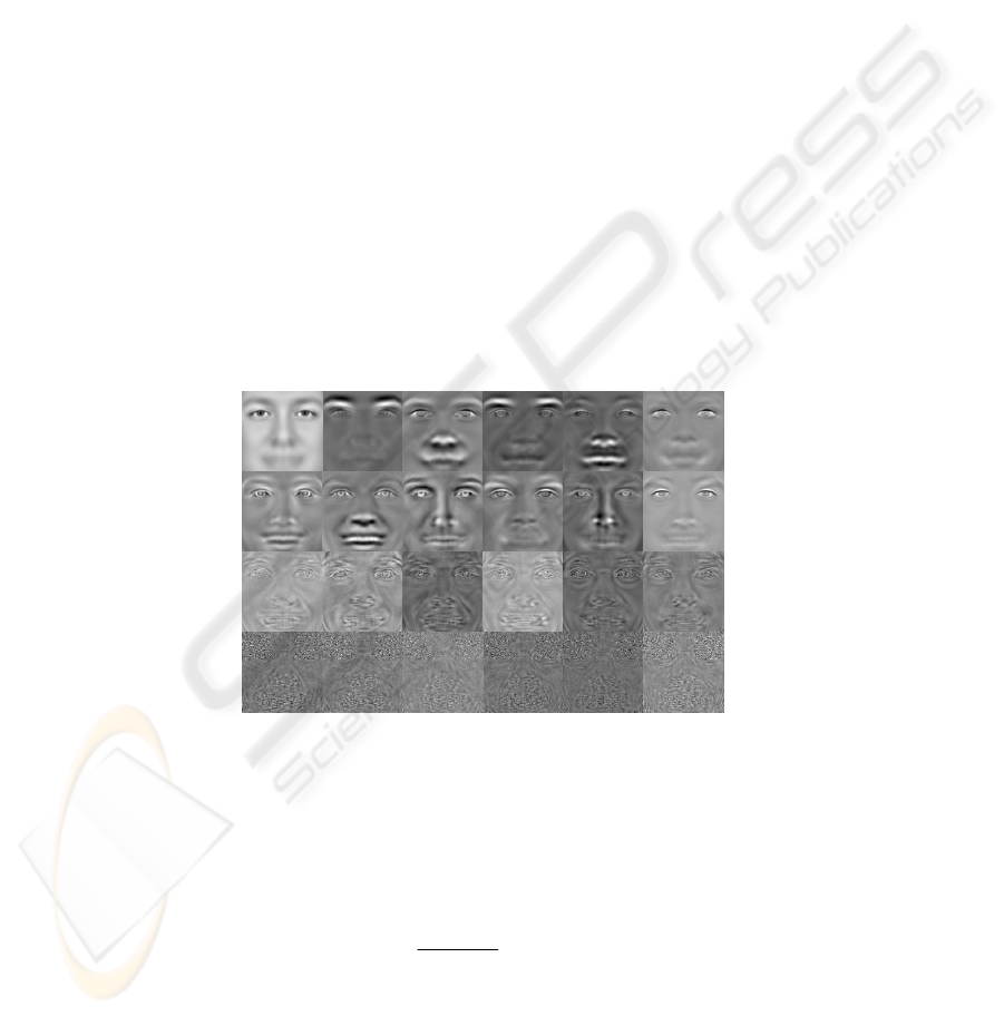
denotes the total scatter matrix. Figure 1 shows examples of Eigenfaces
generated from the generic training images of FRGC data after normalization of the
face images.
Fig. 1. Eigenfaces generated from the FRGC data sorted by the largest eigenvalues; 1
st
and 2
nd
row images show first 12 eigenvectors, 3
rd
row images show 201 ~ 206 eigenvectors and 4
th
row images show 501~506 eigenvectors with small eigenvalues; Eigenvectors do not look like
human faces can be discarded in order to achieve dimensionality reduction.
The LDA is another commonly used method which determines a set of discriminant
basis vectors so the ratio of the between-class scatter and the within-class scatter is
maximized. The optimal basis vectors can be denoted as
(2)
]...[||maxarg
21 mT
T
W
wwwWSW ==
opt
W
]...[
||
||
maxargW
21opt m
W
T
B
T
W
www
WSW
WSW
==
16
where
B
S and
W
S indicate the between-class scatter matrix and the within-class scatter
matrix, respectively. The solution can be solved by the generalized eigenvalue
problem,
(3)
and the final solution becomes the standard eigenvalue problem if S
w
is invertible.
(4)
Due to the fact that the number of training images is smaller than the number of pixels,
the within-class scatter matrix S
w
is singular causing problems for LDA. Fisherfaces
first performs PCA to reduce the dimensionality and thus overcome this singular-
matrix problem and applies LDA in the lower-dimensional subspace. The projection
vectors from Fisherfaces are given as follows.
(5)
where c is the total number of class.
On the other hand, the DLDA derives eigenvectors after simultaneous diagonalization
8. Unlike previous approaches, the DDLA diagonalizes
B
S
first and then
diagonalizes
W
S which can be shown as follows
Λ==
T
W
T
B
WWSIWWS ,
(6)
The smallest eigenvalues in the
B
S
can be discarded since they contain no
discriminative power, while keeping small eigenvalues in the
W
S , especially 0’s.
On the other hand, the GSLDA method avoids inverse or diagonalization approaches
in LDA. The GSLDA approach calculates the orthogonal basis vectors in
(7)
where indicate the null spaces and the upper bars indicate the
orthogonal complement spaces of S
T
and S
w
, respectively. The GSLDA method has
been seen to offer better performance over Fisherfaces and other LDA methods 4, and
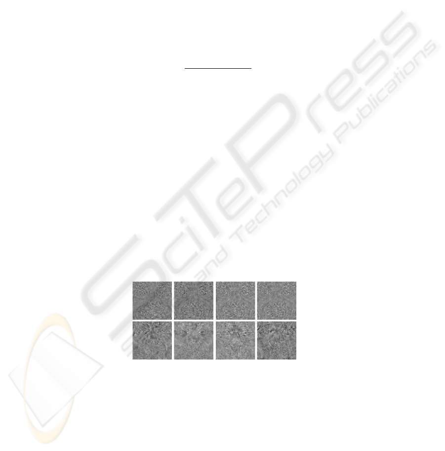
LDA methods typically outperform PCA based methods 2. Figure 2 shows examples
of the LDA basis vectors generated from the generic training images of the FRGC
data.
Fig. 2. The LDA basis vectors; 1
st
row images are examples of the Fisherfaces, and 2
nd
row
images are examples of the GSLDA eigenvectors.
2.1 Advanced Correlation Filters
Correlation filter approaches represent the data in the spatial frequency domain. One
of the most popular correlation filters, the minimum average correlation energy
(MACE) 7 filter is designed to minimize the average correlation plane energy
,...m,iwSwS
iWiiB
21,
=
=
λ
iiiBW
wwSS
λ
=
−1
)0(),0(
WT
SS
]...[
||
||
maxarg
121 −
==
c
pcaW
T
pca
T
pcaB
T
pca
T
W
www
WWSWW
WWSWW
opt
W
]...[||maxarg
21 cNT
T
pca
wwwWSWW
−
==
)0()0(
________
WT
SS ∩
17

resulting from the training images, while constraining the value at the origin to pre-
specified values. Correlation outputs from MACE filters typically exhibit sharp peaks
making the peak detection and location relatively easy and robust. The closed form
expression for the MACE filter vector h is
uΧDΧΧDh
-1-1 1
)(
−+
=
(8)
where X is a d
2
xN complex matrix and its ith column contains the lexicographically
re-ordered version of the 2-D Fourier transform of the ith training image. D is a
d
2
xd
2
diagonal matrix containing the average power spectrum of the training images
along its diagonal and u is pre-specified values. Optimally trading off between noise
tolerance and peak sharpness produces the optimal trade-off filters (OTF). OTF
filter vector is given by
11
()
−+−−
=
1
hTXXTX u
(9)
where
()
2
1
αα
=+−TD C
, 0 ≤
α
≤ 1 , and C is a d
2
xd
2
diagonal matrix whose diagonal
elements C(k,k) represent the noise power spectral density at frequency k. Varying
allows us to produce filters with optimal tradeoff between noise tolerance and
discrimination. It is important to note that when
α
=1, the optimal tradeoff filter
reduces to the MACE filter in eq. (8) and when
α
=0, it simplifies to the noise-tolerant
filter in eq. (9). Large peaks denote good match between the test input and the
reference from which the filter is designed. Due to built-in shift invariance and
designed distortion tolerance, correlation filters for biometric verification exhibit
robustness to illumination variations and other distortions 5.
2.2 Support Vector Machines (SVM)
Support Vector Machines 91011 have been successfully applied in the field of object
recognition, often utilizing the kernel trick for mapping data onto higher-dimensional
feature spaces. The SVM finds the hyperplane that maximizes the margin of
separation in order to minimize the risk of misclassification not only for the training
samples, but also for better generalization to the unseen data.
Unlike PCA and LDA methods where the basis vectors are obtained after centering
the data by either the global mean or the individual mean of the class, the SVM does
not require centering the data. Instead, the SVM emphasizes the data close to the
decision boundary, and the projection coefficients can be estimated by the weight
vector w and bias b. Formally, the decision boundary vector w can be obtained by
minimizing the following known as the Primal Lagrangian form.
(10)
where w is the weight vector orthogonal to the decision boundary and b, N, y,
indicate the bias, the total number of data, and the decision value respectively, and α
i
are the Lagrange multipliers. After differentiation of L respect to w and b, eq. 10 can
be represented by the following the Dual Lagrangian form.
(11)
∑
=
−+−=
N
i
i
T
ii
T
bxybL
1
]1)([2/1),,( wwww
αα
∑∑∑
===
><−=
N
i
N
i
N
j
jijijii
xxyyabL
111
,
2
1
),,(
ααα
w
18
We can also replace with using the kernel trick. The solution
vector w can be denoted as follows depending on whether kernels are applied or not.
(12)
2.3 Challenges in Face Recognition
Unfortunately, the best set of features and algorithms to recognize human faces are
still unknown and many face recognition methods are being developed and evaluated.
The face recognition grand challenge (FRGC) program [12] is aimed at an objective
evaluation of face recognition methods under different conditions, especially in
experiment 4. This experiment 4 is aimed at comparing controlled indoor still images
to uncontrolled (corridor lighting) still images.
The baseline performance from Eigenface method on this data set is 12% verification
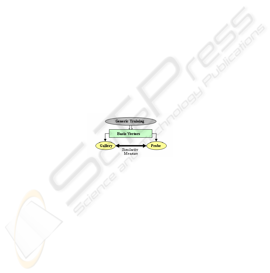
rate (VR) at a false accept rate (FAR) of 0.1%. Figure 3 shows an overview of the
FRGC experiment 4. The generic training set contains 12,776 images (from 222
subjects) taken under controlled and uncontrolled illumination. The gallery set
contains16, 028 images (from 466 subjects) under controlled illumination while the
probe set contains 8014 images (from 466 subjects) under uncontrolled illumination.
Instead of generating basis vectors from the gallery sets, the participants in the FRGC
are supposed to generate basis vectors from the generic training set to assess the
generalization power. Then, the dimensionality of the gallery images and probe
images can be reduced via the basis vectors. Finally, the matching score between
gallery and probe sets needs to be presented to assess the performance.
Fig. 3. An overview of the FRGC experiment 4.
The LDA based methods offer the potential produce better performance over
Eigenfaces. However, the LDA based vectors may not have generalization power to
the unseen classes, since they are optimized based on classes shown previously. This
problem also occurs when we apply the correlation filters since the typical design of
correlation filters is based on the gallery images. The class-dependence feature
analysis (CFA) is proposed to generalize the correlation filters as explained in the
next subsection.
3 Class Dependence Feature Analysis (CFA)
In CFA approach, one filter (e.g., MACE filter) is designed for each class in the
generic training set. Then a test image y is characterized by the inner products of that
test image with the n MACE filters, i.e.
><
ji
xx ,
>
Φ
Φ
<
)(),(
ji
xx
∑∑
==
Φ==
N
i
N
i
iiiiii
xyxy
11
)(,
αα
ww
19
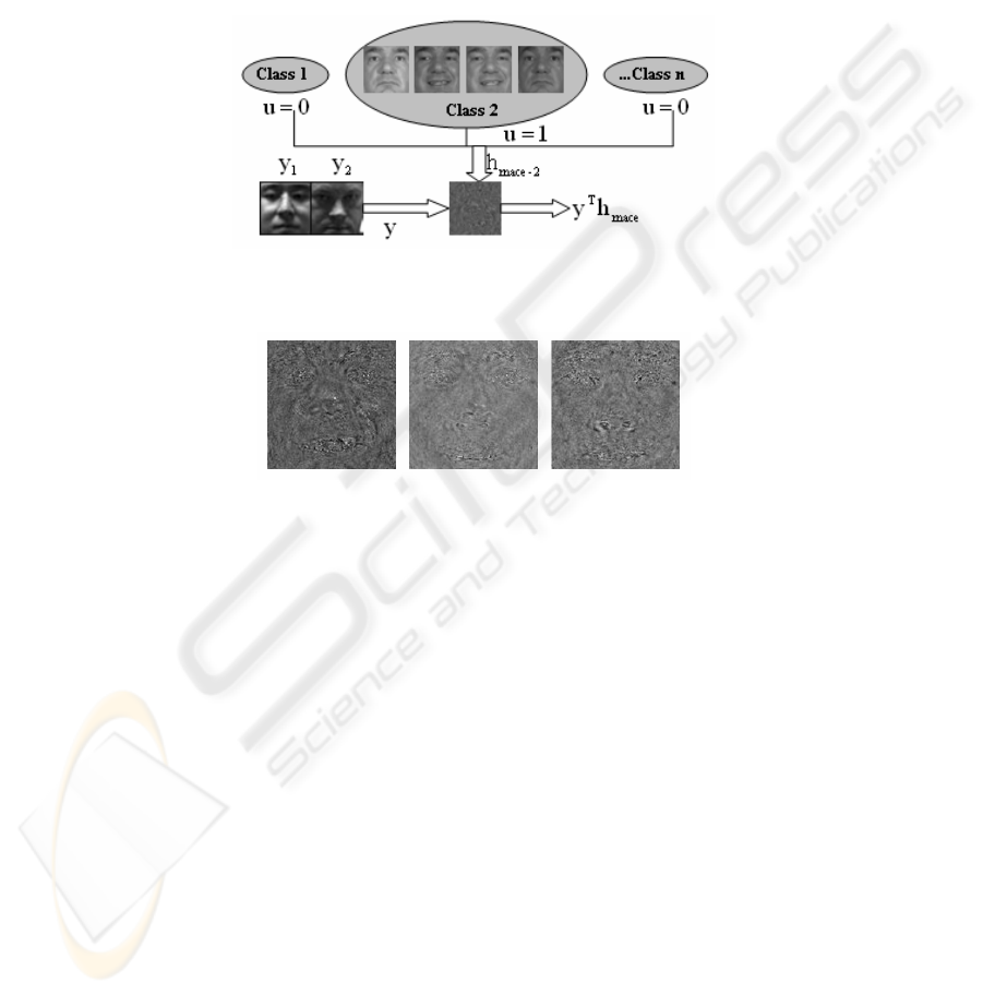
(13)
where h
mace-n
is a filter gives small correlation output for all classes except for class-n.
For example, the number of filters generated by the FRGC generic training set is 222
since it contains 222 classes. Then each input image y is projected onto those basis
vectors and x contains the projection coefficients with the dimensionality of 222.
Then the similarity of the probe image to the gallery image is based on the similarity
between the corresponding class-dependent feature vectors. Figure 2 shows examples
of the CFA basis vectors generated from the FRGC generic training data.
Fig. 4. The CFA algorithm; the filter response of y
1
and h
mace-2
can be distinctive to that of y
2
and h
mace-2
.
Fig. 5. The CFA basis vectors for dimensionality reduction.
3.1 Nonlinear Feature Representation
Due to the nonlinear distortions in human faces, the linear subspace methods have not
performed well in real face recognition applications. As a result, the PCA and LDA
algorithms are extended to represent nonlinear features efficiently by mapping onto a
higher dimensional space. Since nonlinear mappings increase the dimensionality
rapidly, kernel approaches are used as they enable us to obtain the necessary inner
products without computing the actual mapping on to the high dimensional space.
Kernel Eigenfaces and Kernel Fisherfaces 13 are proposed to overcome this problem
using the Kernel PCA and Kernel Discriminant Analysis (KDA) 14. The mapping
function can be denoted as follows.
(14)
Kernel functions defined by can be used without having to
form the mapping as long as kernels form an inner product and satisfies Mercer’
theorem 14. Polynomial kernel (
p
babaK )1,(),( +><=
), Radial Basis Function style
yy ]...[
n-mace2-mace1-mace
T
hhhHx ==
FR
N
→Φ :
>
Φ
Φ
=
< )(),(),( yxyxK
20

kernel (
)2/)(exp(),(
22
σ
babaK −−=
), and Neural Net style Kernel
(
),tanh(),(
δ
−><= bakbaK
) are widely used.
3.2 Kernel CFA (KCFA)
The Kernel CFA algorithm can be extended from the linear CFA method using the
kernel tricks. The correlation output of a filter h and an in
p
ut y can be expressed as
(15)
where
XDX
0.5 ' −
=
indicates pre-whitened version of
X
. From now on, we assume
the
X
is already pre-whitened. After mapping onto a high dimension space, the
solution becomes
(16)
These MACE filters based kernel approaches can be extended to include noise
tolerance as in eq. 9. By replacing D by T, where
(
)
2
1
αα
=+−TD C
, the new kernel
OTF filters show some noise tolerance depending the parameter
α
. The resulting
output for the KCFA approaches can be thought as correlation output in the high
dimensional space with tolerating some level of distortions.
3.3 Experimental Results
The performance of a face recognition algorithm can be measured by its false
acceptance rate (FAR) and its false rejection rate (FRR). FAR is the percentage of
imposters wrongly matched. FRR is the fraction of valid users wrongly rejected. A
plot of FAR vs FRR (as matching score threshold is varied) is called a receiver
characteristic (ROC) curve. The verification rate (VR) is 1-FRR, often the ROC may
show VR vs. FAR. Since the FAR can be more problematic in practical face
recognition applications, the FRGC program compares the verification rates at 0.1 %
FAR. Figure 6 shows the experimental results using Eigenfaces (PCA), GSLDA,
CFA, and KCFA of the experiment 4 of the FRGC. The performance of Eigenfaces is
provided by the FRGC teams. The similarity or distance measure between gallery
image and probe image is important. Commonly used distance measures are L1-norm,
L2-norm 6 and Mahalanobis distance. Those distance measures may not perform well
depending on different algorithms. The normalized cosine distance (given below)
exhibits the best results on the CFA and KCFA.
||)y|| ||xy)/(||-(xy)d(x,
⋅
=
(17)
where d denotes the similarity (or distance) between x and y. Based on the similarity
measure, the identities are claimed using the nearest neighbour rule. The PCA and
GSLDA use the L2-norm while the CFA and KCFA use the distance in eq. 17, and
the resulting performance is shown in Figure 6.
u
uX))XX))(yh)
1
1
−
−
=
Φ⋅ΦΦ⋅Φ=Φ⋅Φ
),(),(
()(()((()(
jii
xxKxyK
y
uXXX
uX)DXDXDD
uX)DX(XDh
'''
0.5-0.5-0.5-0.5-
-1-1-1
1'
1
))((
)(()(
−
+
⋅⋅=
⋅⋅=
⋅=⋅
y
y
yy
-
21
0
0,1
0,2
0,3
0,4
0,5
0,6
Ex p 4
Verification Rates
PCA
GSLDA
CFA
KCFA
Fig. 6. The performance comparisons of the FRGC experiment 4 at 0.1 % FAR. The Kernel
CFA shows the best results over all linear methods.
4 Distance Measure in SVM Space
If we can design a decision boundary to separate one face class (with all its
distortions) from all other classes, we can achieve robust face recognition in real
applications. However, it is not an easy task to design those decision boundaries
under all possible distortions. Therefore, a direct use of the SVM as a classifier may
produce worse performance under those distortions since only small number of
training images are allowed to build the SVM. In stead of using the SVM as a
classifier directly, we use the projection coefficients of KCFA features in the SVM
space. Figure 7 shows an example of the decision boundary and distance measure in
the SVM space.
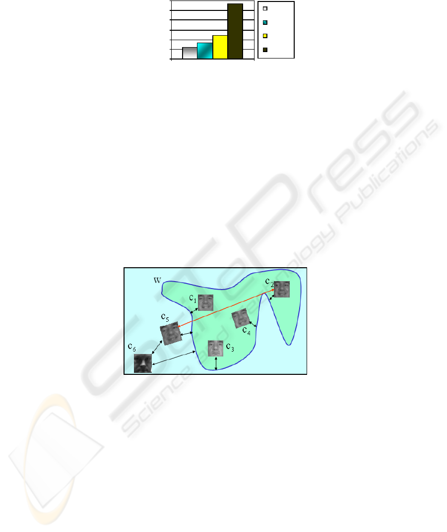
Fig. 7. The decision boundary of a class and distance measure in the SVM space; A direct use
of the SVM may falsely indicate that image C
5
as not the same person with those images inside
the decision boundary.
The L2-norm distance without the SVM decision boundary w may be large between
the same classes causing poor performance. In this case, the L2-norm distance of C
2
and C
5
is greater than that of C
6
and C
5
causing a misclassification. However, if we
project C
5
on to w, the projection coefficients among the same classes will be small
and we can change the threshold distance depending on FAR and FRR. Thus this
approach may lead to flexibility of varying thresholds and better performance in
classification. We apply linear machines, RBF and Polynomial Kernels (PK) in order
to find the best separating vectors varying parameters associated with each kernel
method. The nonlinear SVM such as RBF and PK show better performance over the
linear SVM.
22
Building the SVM of the face images (of size 128x128 pixels) without any form of
dimensionality reduction is an extremely challenging task. Since the dimensionality
reduction based on KCFA is better than other approaches, we use KCFA features
(222 features) as an input for building the SVM. We design 466 SVMs (in a one-
against all framework) using the gallery set of the FRGC data. The probe images are
then projected on the class-specific SVMs which will provide a similarity score. As
shown in Figure 8, the new distance measure in the SVM space produces better
results than using normalized cosine distance. We also compared the different kernel
approaches such as KPCA and KDA with different distance measure showing the
SVM based KPCA methods have superior to other kernel approaches as shown in
Figure 9.
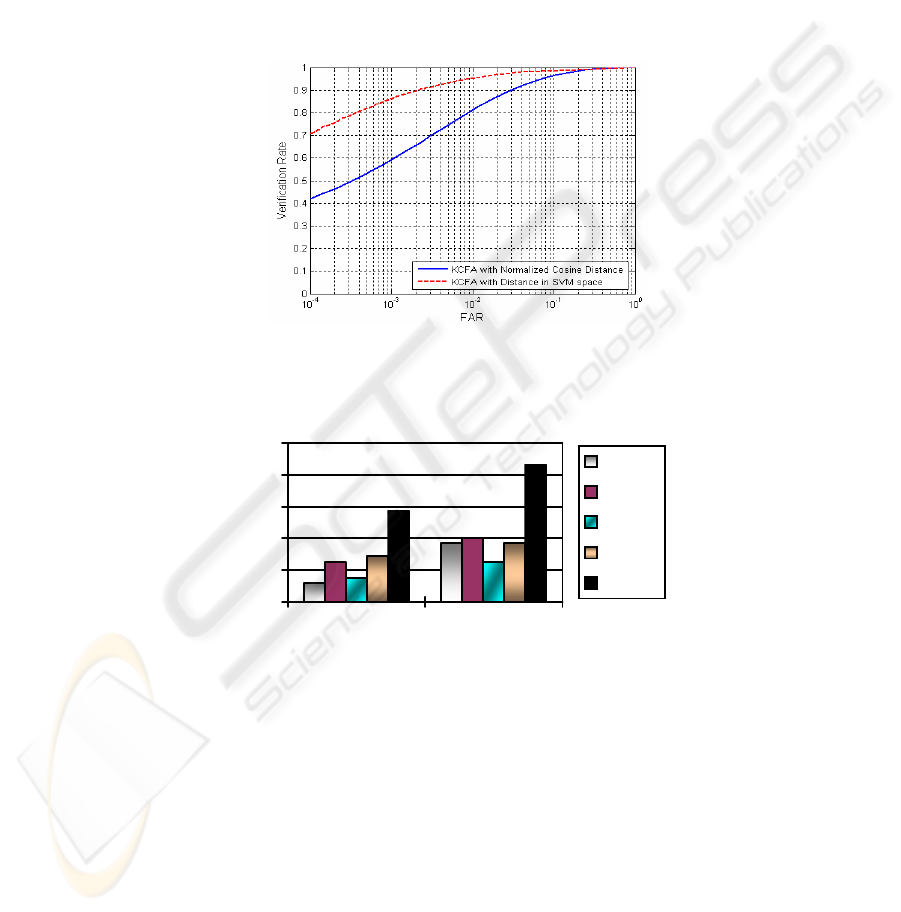
Fig. 8. VR vs FAR for FRGC experiment 4 for different methods using normalized cosine
distances and SVM space.
0
0,2
0,4
0,6
0,8
1
Normalized Cosine L2-SVM Space
Verfication Rates
PCA
KPCA
GSLDA
KDA
KCFA
Fig. 9. VR vs FAR for FRGC experiment 4 using KCFA with different distance measure.
5 Conclusions
Due to nonlinear distortions coupled with blurry images on face images, linear
approaches such as PCA, LDA, and CFA may not represent nor discriminate facial
features efficiently. By using kernel tricks, the Kernel CFA performs dimensionality
reduction showing better performance over all linear approaches. After reducing the
dimensionality of the data, we map the data again onto higher dimension spaces to
23

build the decision boundaries which separate a class from all classes. Since direct
mapping onto a high dimension using high quality normalized faces (128 by 128
pixels) will be not an easy task, dimension reduction scheme may be necessary before
mapping onto higher dimension where the non-linear features are well represented.
By incorporating the SVM for a new distance measure, the performance gain is
dramatic. These approaches (KCFA, Distance in the SVM space) can be extended
further by adding more databases and may perform robust face recognition in real
applications. Our ongoing work will be conducting the comparison our approaches on
large scale database containing pose changes as well.
References
1. M. Turk and A. Pentland, “Eigenfaces for Recognition,” Journal of Cognitive
Neuroscience, Vol. 3, pp.72-86, 1991.
2. P.Belhumeur, J. Hespanha, and D. Kriegman, “Eigenfaces vs Fisherfaces: Recognition
Using Class Specific Linear Projection,” IEEE Trans. PAMI, Vol.19. No.7, pp.711- 720,
1997.
3. L.F. Chen, H.Y.M. Liao, M.T. Ko, J.C. Lin, and G.J. Yu, “A new LDA-based face
recognition system which can solve the small sample size problem,” Pattern Recognition,
Vol. 33, pp. 1713-1726, 2000
4. W. Zheng, C. Zou, and L. Zhao, “Real-Time Face Recognition Using Gram-Schmidt
Orthgonalization for LDA,” IEEE Conf. Pattern Recognition (ICPR) , pp.403-406, 2004
5. M. Savvides, B.V.K. Vijaya Kumar and P. Khosla, “Face verification using correlation
filters,” Proc. Of Third IEEE Automatic Identification Advanced Technologies, Tarrytown,
NY, pp.56-61, 2002.
6. C. Xie, M. Savvides, and B.V.K. Vijaya Kumar, “Redundant Class-Dependence Feature
Analysis Based on Correlation Filters Using FRGC2.0 Data,” IEEE Conf. Computer Vision
and Pattern Recognition(CVPR) , 2005
7. A. Mahalanobis, B.V.K. Vijaya Kumar, and D. Casasent, “Minimum average correlation
energy filters,” Appl. Opt. 26, pp. 3633-3630, 1987.
8. K. Fukunaga, “Introduction to Statistical Pattern Recogniton (2
nd
Edition)”, New
York:Academic Press, 1990
9. V. N. Vapnik, The Nature of Statistical Learning Theory, New York: Springer-Verlag,
1995.
10. B. Schölkopf, Support Vector Learning, Munich, Germany: Oldenbourg-Verlag, 1997.
11. P. J. Phillips, “Support vector machines applied to face recognition,” Advances in Neural
Information Processing Systems 11, M. S. Kearns, S. A. Solla, and D. A. Cohn, eds., 1998.
12. P. J. Phillips, P. J. Flynn, T. Scruggs, K. W. Bowyer, J. Chang, K. Hoffman, J. Marques, J.
Min, and W.Worek, "Overview of the Face Recognition Grand Challenge,” IEEE Conf.
Computer Vision and Pattern Recognition(CVPR), 2005
13. M.H Yang, “Kernel Eigenfaces vs. Kernel Fisherfaces: Face Recognition using Kernel
Methods,” IEEE Conf. Automatic Face and Gesture Recognition, pp. 215-220, 2002
14. K.R. Muller, S.Mika, G. Ratsch, K. Tsuda, and B. Scholkopf , “An Introduction to Kernel-
Based Learning Algorithms,” IEEE Trans. Neural Network, Vol.12, No.2, pp.181-202, Mar
2001.
24
