
DECISION SUPPORT SYSTEM FOR BREAST CANCER DIAGNOSIS
BY A META-LEARNING APPROACH BASED ON GRAMMAR
EVOLUTION
Albert Fornells-Herrera, Elisabet Golobardes-Rib
´
e and Ester Bernad
´
o-Mansilla
Research Group in Intelligent Systems
Enginyeria i Arquitectura La Salle, Ramon Llull University. Quatre Camins 2, 08022 Barcelona (Spain)
Joan Mart
´
ı-Bonmat
´
ı
Computer Vision and Robotics Group
University of Girona. Avda. Llu
´
ıs Santal
´
o s/n, 17071 Girona (Spain)
Keywords:
Breast Cancer Diagnosis, Strategic Decision Support Systems, Evolutionary Programming, Meta-Learning,
Application of Artificial Intelligence on Medicine.
Abstract:
The incidence of breast cancer varies greatly among countries, but statistics show that every year 720,000 new
cases will be diagnosed world-wide. However, a low percentage of women who suffer it can be detected using
mammography methods. Therefore, it is necessary to develop new strategies to detect its formation in early
stages. Many machine learning techniques have been applied in order to help doctors in the diagnosis decision
process, but its definition and application are complex, getting results which are not often the desired.
In this article we present an automatic way to build decision support systems by means of the combination
of several machine learning techniques using a Meta-learning approach based on Grammar Evolution (MGE).
We will study its application over different mammographic datasets to assess the improvement of the results.
1 INTRODUCTION
Breast cancer is the most common cancer among
western women and is the leading cause of cancer-
related death in women aged 15-54. Screening pro-
grams have proved to be good practical tools for pre-
maturely detecting and removing breast cancer, and
increasing the survival percentage in women (Win-
fields et al., 1994). In an attempt to improve early
detection, a number of Computer Aided Diagnosis
(CAD) techniques have been developed. There are
several approaches to CAD, but we focus on the breast
cancer diagnosis using mammographic images. A
mammographic image is processed in order to iden-
tify the microcalcifications (µCa) that appear. Hu-
man experts agree on their relevance in diagnosing a
new case. After characterizing the µCa through a set
of features, we diagnose each image using machine
learning techniques. Previous studies applying ma-
chine learning techniques found that these techniques
improved the accuracy rate (in terms of correct clas-
sifications) but decreased the reliability rate (in terms
of robustness and stability) compared to human ex-
perts (Golobardes et al., 2002). Our purpose is to
improve the reliability rate so experts can have more
confidence in the results, when they need to decide
whether a sample is benign or malign.
When people make critical decisions, they usually
take into account the opinions of several experts rather
than relying on their own judgement or that of an only
trusted advisor. Therefore, an obvious approach for
making more reliable decisions is to combine the out-
put of several models/classifiers by means of a meta-
level, which coordinates the decision support system.
Although a 100% of reliability is not assured, the con-
fidence in the results is usually increased.
However, models’ combination has the disadvan-
tage of being rather hard to design as it is not easy
to intuitively understand what factors are contribut-
ing to the different predictions. An automatic process
that searched for the best combination of single clas-
sifiers would help in the design process. In this pa-
per, we propose an automatic way of defining deci-
sion support systems using a Meta-learning approach
based on Grammar Evolution (MGE). Grammar Evo-
lution (GE) (Ryan et al., 1998) is a variant of Evolu-
tionary Computation (EC) (Goldberg, 1989) designed
to find algorithms using a genotype to fenotype map-
ping process by means of a Backus Naur Form (BNF)
grammar, which leads the searching process. We
adapt a GE to guide the search to the most reliable
schema of classifier combinations. Also, the result-
222
Fornells-Herrera A., Golobardes-Ribé E., Bernadó-Mansilla E. and Martí-Bonmatí J. (2006).
DECISION SUPPORT SYSTEM FOR BREAST CANCER DIAGNOSIS BY A META-LEARNING APPROACH BASED ON GRAMMAR EVOLUTION.
In Proceedings of the Eighth International Conference on Enterprise Information Systems - AIDSS, pages 222-229
DOI: 10.5220/0002492202220229
Copyright
c
SciTePress

ing meta-learning approach will be applied to breast
cancer diagnosis.
This article is organized as follows. Section 2 sur-
veys some related work. Section 3 sets the back-
ground of classifier combination, and defines the main
structure of our meta-learning approach (MGE). Sec-
tion 4 describes the particular setting of MGE for the
breast cancer diagnosis problem. Next, Section 5 an-
alyzes the results and finally, we summarize conclu-
sions and further work in section 6.
2 RELATED WORK
Several decision support systems have been applied
to perform the diagnosis of breast cancer using the
µCa extracted from mammographic images. Some
of them are Support Vector Machines (Campani
et al., 2000), Nearest-Neighbour algorithms (Kauff-
man et al., 2000), Bayesian Networks (Edwards et al.,
2000) or Fuzzy Neural Networks (Cheng et al., 1998).
We have been working successfully with different
Artificial Intelligence (AI) techniques such as Genetic
Algorithms (GA) (Goldberg, 1989) and Case Base
Reasoning (CBR) (Aamodt and Plaza, 1994) to tackle
this problem (Garrell et al., 1999) (Golobardes et al.,
2002). However, we prefer to focus in a CBR ap-
proach because it allows experts to get an explana-
tion of its classification (malign or benign) in terms
of the most similar cases. In these previous works,
the results were compared with the classifications by
human experts (Mart
´
ı et al., 2000). The conclusions
were that AI techniques improved the accuracy rate
but the reliability rate was decreased. One of the rea-
sons was the difficulty of defining a reliable similarity
function for CBR.
In (Golobardes et al., 2001) a Genetic Program-
ming (GP) (Koza, 1992) approach was used as an
automatic process for designing similarity functions
for CBR. The system found a similarity function that
improved the previous results, but they were still not
good enough. The reason was attributed to the huge
search space in which the GP had to find the solu-
tion. In (Fornells et al., 2005b) a new approach based
on GE and CBR was proposed to reduce the search
space, by the use of a grammar that led the search
process. The comparison of the GP-CBR approach
and the GE-CBR approach showed that the GE-CBR
approach works better if the grammar is well defined
(Fornells et al., 2005a).
Combining multiple models is a popular research
topic in machine learning research. The most im-
portant methods for combining models are bagging
(Breiman, 1996a), boosting (Schapire et al., 1997)
and stacking (Wolpert, 1990). Bagging and boosting
are based in the combination of their outputs using
voting schemes. The difference between them is that
boosting uses a weighting vote. On the other hand,
Stacking was introduced by Wolpert (Wolpert, 1990)
in the neural network literature, and it was applied to
numeric prediction by Breiman (Breiman, 1996b). It
is a technique based on a meta-level that makes deci-
sions using heuristics which combine the outputs of
several classifiers. Later, Ting and Witten (Ting and
Witten, 1997a) compared different meta-level mod-
els empirically and found that a simple linear model
performs best. Also, they demonstrated the advan-
tage of using the probabilities of classifier predictions
as meta-level data. A combination of stacking and
bagging was also investigated in (Ting and Witten,
1997b). Many different models were generated by
varying the learning parameters (Oliver and Dowe,
1995) (Kwok and Carter, 1990) and by using differ-
ent sampling methods (Freund and Schapire, 1996)
(Ali and Pazzani, 1996).
In (Vallesp
´
ı et al., 2002) these concepts were used
to define several meta-levels by means of heuristics
based on the results of different machine learning
techniques over the mammography dataset proposed
in (Mart
´
ı et al., 2000). Nevertheless, this way of defin-
ing meta-levels is very limited. For this reason, we
propose MGE as an automatic way of defining meta-
levels, and we study its application over new and im-
proved datasets of breast cancer diagnosis.
3 MGE: META-LEARNING
APPROACH BASED ON
GRAMMAR EVOLUTION
3.1 Meta-learning
Meta-learning can be defined as learning from infor-
mation generated by a(some) learner(s). It can also be
viewed as learning meta-knowledge from the learned
information. Therefore, it is a general technique to
coalesce the results of multiple classifiers.
It requires at least two levels: A level composed
by a set of trained classifiers (level-0 model) using a
subset of the original dataset (level-0 data), and an-
other level trained (level-1 model) using the outputs
of the level-0 models (level-1 data). (Breiman, 1996a)
demonstrated that the combination of all the model-0
outputs usually improves the results of the individual
classifiers.
Level-0 models can be of two types: (1) Heteroge-
neous (the classifiers used are different) and (2) Ho-
mogeneous (all the classifiers used are equal). In turn,
level-0 data can be distributed by each classifier in
several ways: (1) Duplicating all the samples, (2) Dis-
tributing samples clustered in disjoint subsets, or (3)
DECISION SUPPORT SYSTEM FOR BREAST CANCER DIAGNOSIS BY A META-LEARNING APPROACH
BASED ON GRAMMAR EVOLUTION
223
Distributing samples clustered in subsets allowing the
repetition of the samples. Breiman (Breiman, 1996a)
exposed that it is desired to level-0 models to be un-
stable, which means that they should be easily altered
if their training dataset is altered. Nevertheless, Ting
and Witten in (Ting and Witten, 1997b) demonstrated
that it is not necessary. However, they both agree
that the level-0 design process is critical in the sense
that all classifiers must complement each other, that
is, they need to cover all the possible solutions.
The first difficulty in the level-1 design process is
to define what data from the output of level-0 clas-
sifiers should be used: (1) Only the class predicted
(Breiman, 1996a), (2) The class predicted and the
most similar samples (Chan and Stolfo, 1993), or (3)
the probabilities of belonging to each possible class
(Ting and Witten, 1997a). Option (1) does not al-
low level-1 model to get any measure of the confi-
dence on the whole prediction. Although option (2)
adds extra information using the internal information
of level-0 models, it is difficult to integrate differ-
ent internal representations. On the other hand, op-
tion (3) provides level-1 model information on the
confidence in all the class predictions, which can be
used to better evaluate the behaviour of the level-0
models. Nevertheless, the selection of the type of
information used as level-1 data is conditioned by
the level-1 model. There are several ways of im-
plementing the level-1, of which the most impor-
tant are: (1) Manual heuristics defined by an expert,
(2) Voting schemas (Breiman, 1996a), (3) Weighting
voting schemas (Schapire et al., 1997), (4) Arbiter
strategy based on solving conflicts (Chan and Stolfo,
1993), (5) Lineal regressions schemes (Ting and Wit-
ten, 1997a) and (6) Inductive and explanation-based
learning (Flann and Dietterich, 1989).
We can see that meta-learning allows the definition
of a hierarchy, which can be used to model a decision
support system.
3.2 Grammar Evolution
GE (Ryan et al., 1998) is a technique based on Evo-
lutionary Computation (EC), where a BNF grammar
is used in a genotype to fenotype mapping process in
order to transform the individual (represented by an
array of bits) into an executable program or function.
The fitness is assigned depending on the result of the
program.
The BNF grammar is composed by a tuple {N, T, P,
S}. N and T represent the set of non-terminals and ter-
minals respectively, S is the starting production, and
P defines the rules for each production of the non-
terminals. At the beginning of the mapping process,
each individual has a program represented by the non-
terminals of the starting production. The first step
consists of clustering the bits of the individual in inte-
1th Model
.....
GE
Level-0
Models
Level-1
Model
Level-0
Data
Level-1
Data
New Problem
Individual Predictions
Kth
Model
Combined Prediction
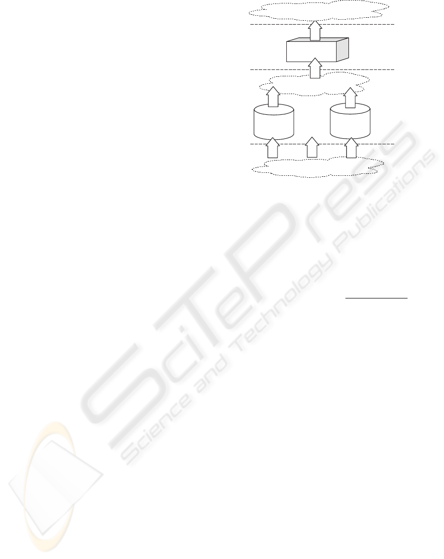
Figure 1: Evaluation of an individual in MGE.
gers of X bits called codons, where X depends on the
production with more rules. Next, the non-terminals
elements are iteratively replaced by the elements of
one rule of the same production, which is selected us-
ing the codons of the individuals by the equation:
new rule = modulus of
actual codon
number of rules
(1)
This process is repeated until all the elements of the
program are terminals, and therefore the program can
be run. If the codons have run out and the mapping
process has not ended, then a wrapping operator is
applied. It means that codons are reused again from
the beginning.
3.3 Definition of Meta-levels by
Means of GE
Subsection 3.1 describes the term meta-learning as
a system which learns from other learning systems.
Nevertheless, it is not trivial to define how to com-
bine the output of the level-0 models to get the level-1
model. For this reason, we want to automate it using
the GE approach, which needs the definition of the
BNF grammar and the evaluation of the individuals.
The BNF grammar can be defined as an expression
that represents a linear regression, a set of rules, or
any way of combining the outputs of several level-0
models. This variety allows GE more flexibility.
Figure 1 shows the evaluation of a sample by an in-
dividual (a potential meta-level), which consists of:
(1) Translation of the individual into an expression
modeled by the BNF grammar, (2) Test the sample
in all level-0 models in order to get the level-1 data,
(3) The last predictions are replaced in the expression
ICEIS 2006 - ARTIFICIAL INTELLIGENCE AND DECISION SUPPORT SYSTEMS
224

Table 1: Characteristics of the datasets studied.
Dataset Attr. Class Distribution
Wisconsin 10 benign (458), malign (241)
µCa 22 benign (121), malign (95)
DDSM 143 b1(61), b2(185), b3(157),
b4(98)
MIAS-Birads 153 b1(128), b2(78), b3(70),
b4(44)
MIAS-3C 153 fatty(106), dense(112),
glandular(104)
to get the combined prediction. Finally, the fitness of
the individual is computed using the statistics over all
the tested samples.
4 SETTING MGE FOR THE
PROBLEM
4.1 Datasets
We applied our approach to different datasets re-
lated with breast cancer diagnosis (see Table 1).
The Wisconsin dataset comes from UCI repository
(Blake and Merz, 1998) and the rest of the them
belong to our own repository. These are mammo-
graphic images digitalized by the Computer Vision
and Robotics Group from the University of Girona.
The µCa dataset (Mart
´
ı et al., 2000) contains sam-
ples from Trueta Hospital (in Girona), while DDSM
(Heath et al., 2000) and MIAS (Suckling et al., 1994)
are public mammographic images datasets, which
have been studied and preprocessed in (Oliver et al.,
2005b) (Oliver et al., 2005a) respectively. The µCa
dataset contains samples of mammographies previ-
ously diagnosed by surgical biopsy, which can be be-
nign or malign. DDSM and MIAS-Bi classify mam-
mography densities, which was found relevant for the
automatic diagnosis of breast cancer. Experts clas-
sify them either in four classes (according to BIRADS
(Samuels, 1998) classifications) or three classes (clas-
sification used in Trueta Hospital).
4.2 Level-0 Model
As we mentioned previously, we focus in CBR be-
cause it provides an explanation of its classification.
In order to select the most suitable level-0 mod-
els, a previous study testing several techniques is
needed over the different datasets. A self CBR ap-
proach with different configurations was tested with
different similarity functions (Clark, Cosines, Ham-
ming, Euclidean, Cubic) using sample correlation as
weighting schema, and three nearest neighbour tech-
nique in the retrieval phase. Other machine learn-
ing techniques from Weka (Witten and Frank., 2000)
were also tested: IBK (Aha and Kibler, 1991), ID3
(Quinlan, 1986), C4.5 (Quinlan, 1993), PART (Frank
and Witten, 1998), Bayesian Neural Network (BNN)
(Freeman and Skapura, 1991) and Sequential Mini-
mal Optimization (SMO) (Platt, 1998).
N={ <program>, <expression>, <prob>,
<op>, <constant> }
T={if, (, ), else, then, endif, ≥, <, class
1
,...,
class
C
,noclass, P
class
1
K
1
,...,P
class
C
K
K
}
S={<program> }
P=
<program> ← <expression>
<expr.> ← if (<prob><op><constant>) then
<expression>
else
<expression>
endif
← class
1
| ...| class
C
| no class
<prob> ← P
class
1
K
1
| ...| P
class
C
K
K
<op> ←≥|<
<constant> ← 0.25 | 0.5 | 0.75
Figure 2: BNF grammar used in GE.
Table 2 summarizes the error rates and the standard
deviation for each dataset. The results were computed
using a 10-fold stratified cross-validation, and using
10 random seeds. Because we want to improve the
results for all datasets, the level-0 models selected are
these which have the lowest error and lowest standard
deviation. They are marked using bold letters.
4.3 Level-1 Model
As we explained in subsection 3.1, the most useful
level-1 data is the probability of belonging to each
possible class. In the CBR approach, it is computed
using the equation proposed by (Ting and Witten,
1997a):
P
i
x =
p
s=1
f(y
s
)/d(x, x
s
)
p
s=1
1/d(x, x
s
)
(2)
where:
x is the new problem to solve
x
s
is the case ’s’ retrieved
d(x, x
s
) is the difference between ’x’ and ’x
s
’
p indicates the number of samples returned
f(y
s
) is ’1’ if i = y
s
, and ’0’ otherwise
The probabilities for the other methods are com-
puted internally by Weka. We define the level-1
data as a list of predictions generated by the sam-
ples tested, where each prediction is composed by the
probabilities of belonging to each possible class (C),
for each level-0 model used.
DECISION SUPPORT SYSTEM FOR BREAST CANCER DIAGNOSIS BY A META-LEARNING APPROACH
BASED ON GRAMMAR EVOLUTION
225

Table 2: % of error and standard deviation using several machine learning over the datasets of the table 1.
Method Wisconsin µCa DDSM MIAS-Bi MIAS-3C
Clark 10.80 (9.23) 34.26 (4.6) 44.71 (6.6) 26.88 (7.15) 22.61 (8.4)
Cosines 34.5 (1.4) 43.98 (9.4) 88.42 (6.74) 85.63 (7.2) 81.37 (9.2)
Hamming 3.43 (1.3) 32.41 (9.54) 55.09 (5.9) 33.13 (6.4) 32.30 (5.9)
Euclidean 3.42 (1.2) 34.72 (7.14) 53.49 (5.6) 29.69 (5.4) 29.19 (6.3)
Cubic 3.41(1.5) 33.38 (7.4) 52.30 (6.4) 32.81 (5.09) 31.06 (5.8)
Ib
K
(k=3) 3.43 (1.3) 30.55 (11.3) 53.29 (9.5) 29.69 (12.3) 27.63 (7.9)
ID3 5.86 (2.5) 35.65 (8.3) 45.70 (6.7) 29.06 (11.7) 32.06 (9.6)
C4.5 5.43 (1.9) 39.81 (10.2) 51.09 (3.5) 31.56 (11.5) 34.16 (8.7)
PART 5.29 (1.9) 38.42 (8.5) 55.88 (7.8) 42.51 (10.12) 34.78 (8.2)
BNN 4.01 (2.4) 36.11 (9.8) 56.48 (5.2) 32.81 (9.3) 29.51 (9.7)
SMO 3.43 (1.6) 31.48 (11.1) 44.11 (5.6) 29.68 (11.6) 25.15(5.2)
Table 3: GE configuration.
Parameter Value
Generation 500
Population 1000
Ending 0.95% of the ideal fitness
Operators Prob. Cross (0.8)
Prob. Repro. (0.2)
Prob. Mutation (0.3)
Max. Wrappring (2)
Selection Tournament (2)
# Codons 200 codons
Evaluation Eq. 3 with statistics from the
level-1 outputs
Initialization Ramped
Replacement Steady-State (SS)
Random Seed 10
Figure 2 represents the grammar that defines the
genotype to fenotype mapping process used to trans-
form the individual into a level-1 model. At the end of
the GE training process, the individual with the best
fitness will be selected as the level-1 model.
The fitness of individuals is computed by equation
3, which is based on the statistic about the accuracy
rate, and unclassified rate from the level-1 outputs:
fitness =0.75 · accuracy − 0.25 · unclassified (3)
Each component has an associated weighting value
that models the individual’s behaviour. Finally, ta-
ble 3 contains the GE configuration used in the meta-
learning searching process.
4.4 Training and Testing the Models
Given a dataset α = {(y
n
,x
n
),n =1..N}, where
y
n
is the class value and x
n
represents the attribute
values of the nth instance. The samples are randomly
split into J equal parts α
1
,...,α
J
. Let’s define α
test
j
and α
train
j
= α − α
test
j
to be the test and training
sets for the jth fold of a J-fold cross-validation. Also,
α
train
j
is split into M equal parts β
1
,...,β
M
. Let’s
define β
test
j,m
and β
train
j,m
= α
train
j
−β
test
j,m
to be the test
and training sets for the mth fold of another M-fold
cross-validation.
Training MGE consists of M training subcycles of
the level-0 models. Each one uses β
train
j,m
as level-0
data and β
test
j,m
to test the level-0 model. The proba-
bilities of belonging to each class are used as level-1
data for the MGE individual that is being evaluated to
obtain the statistics. The average of the M statistics
allows the system to compute the fitness using equa-
tion 3. The MGE final statistics are computed in a
J fold cross-validation, which implies training MGE
with α
train
j
and testing with α
test
j
J times.
It is obvious that this training and testing process
is computationally expensive as the evaluation of one
individual implies several runs of the level-0 mod-
els. Nevertheless, this penalization can be avoided if
all the predictions resulting from all β
train
j,m
and β
test
j,m
∀jin1 ...J ∀min1 ...M are previously computed.
Therefore, the individual’s evaluation only implies the
replacement of the precomputed predictions into the
expression, and running time is drastically decreased.
This way of training and testing the system war-
rants that test folds are independent, and the individ-
ual found by MGE is tested using samples that have
not been used in the training process.
5 RESULTS AND DISCUSSION
Tables 4, 5, 6, 7 and 8 show the error rate (percentage
of missclassifications) and the standard deviation for
the datasets of Table 1 using the experimental set de-
scribed in subsection 4.4. Also, we have applied Bag-
ging (Breiman, 1996a), AdaBoostM1 (Freund and
Schapire, 1996) and Stacking (Wolpert, 1990) from
Weka in order to compare their results.
The results can be analyzed from two points of
view: the improvement of meta-classifiers in compar-
ICEIS 2006 - ARTIFICIAL INTELLIGENCE AND DECISION SUPPORT SYSTEMS
226

ison with the single classifiers, and the MGE improve-
ment with respect to the other meta-classifiers.
The results of a meta-classifier are related with the
results of its level-0 models. Comparing tables 5 - 8
with table 2, we observe that the meta-classifier ap-
proaches do not improve the error rate. Wisconsin
dataset is the exception because the MGE approach
(table 4) improves the results of the level-0 predic-
tions (table 2). This happens because this problem is
less complex than the others. Also, we have applied
a t-test student between the best single-classifiers and
the MGE results, and the improvements are not statis-
tical significant (at 95% confidence level)
12
.
Table 4: % of error and dev. in Wisconsin.
Meta-level Level-0 models Error
MGE Euc., Cub., SMO 2.72 (1.7)
Bagging Ib
3
3.43 (1.6)
Bagging BNN 4.01 (2.5)
Bagging SMO 3.43 (1.9)
AdaBoost Ib
3
3.14 (1.8)
AdaBoost BNN 4.86 (1.9)
AdaBoost SMO 3.43 (1.7)
Sta-Ib
3
Ib
3
, BNN, SMO 3.57 (1.7)
Sta-BNN Ib
3
, BNN, SMO 3.29 (1.4)
Sta-SMO Ib
3
, BNN, SMO 3.57 (1.5)
Table 5: % of error and dev. in µCa.
Meta-
level
Level-0 models Error
MGE Ham., IB3, SMO 32.33 (9.7)
Bagging Ib
3
33.79 (10.3)
Bagging ID3 35.68 (10.8)
Bagging SMO 33.33 (12.1)
AdaBoost Ib
3
33.79 (11.7)
AdaBoost ID3 36.11 (9.9)
AdaBoost SMO 32.48 (11.1)
Sta-Ib
3
Ib
3
, ID3, SMO 39.81 (11.2)
Sta-SMO Ib
3
, ID3, SMO 35.64 (10.5)
Table 6: % of error and dev. in DDSM.
Meta-level Level-0 models Error
MGE Clk., ID3, SMO 47.10 (5.6)
Bagging C4.5, 51.29 (4.5)
Bagging ID3 49.91 (6.4)
Bagging SMO 44.91 (6.3)
AdaBoost C4.5 53.89 (8.3)
AdaBoost ID3 46.31 (4.3)
AdaBoost SMO 42.72 (5.7)
Sta-C4.5 C4.5, ID3, SMO 46.31 (6.2)
Sta-SMO C4.5, ID3, SMO 50.49 (5.9)
1
Sta-XXX means that stacking is applied using XXX as
meta-classifier. ID3 is not supported as meta-classifier in
Weka tool because it only works with nominal values
2
The CBR approach is not supported in Weka tool. We
apply the next best level-0 model
Table 7: % of error and dev. in MIAS-Birads.
Meta-level Level-0 models Error
MGE Clk, Ib
3
, SMO 32.50 (10.6)
Bagging ID3 34.37 (10.8)
Bagging Ib
3
29.71 (11.9)
Bagging SMO 30.93 (12.8)
AdaBoost ID3 38.43 (5.9)
AdaBoost Ib
3
32.82 (11.2)
AdaBoost SMO 33.12 (11.6)
Sta-Ib
3
ID3, Ib
3
, SMO 40.93 (11.8)
Sta-SMO ID3, Ib
3
, SMO 33.43 (10.4)
Table 8: % of error and std. in MIAS-3C.
Meta-level Level-0 models Error
MGE Clk., ID3, SMO 28.57 (4.6)
Bagging Ib
3
30.12 (6.8)
Bagging ID3 30.74 (8.8)
Bagging SMO 23.91 (5.1)
AdaBoost Ib
3
29.81 (8.8)
AdaBoost ID3 38.19 (6.2)
AdaBoost SMO 26.31 (5.1)
Sta-Ib
3
Ib
3
ID3 SMO 33.85 (7.1)
Sta-SMO Ib
3
ID3 SMO 31.98 (6.3)
if ( P
C
2
K
1
< 0.75 ) then Class
1
else if (
P
C
0
K
1
≥ 0.25 ) then if (P
C
2
K
0
< 0.25 ) then Class
0
else Class
1
endif else Class
1
endif endif
Figure 3: Meta-level discovered in Wisconsin.
if ( P
C
1
K
1
≥ 0.75 ) then if ( P
C
0
K
1
≥ 0.50
) then Class
0
else unknown endif else if (
P
C
2
K
1
< 0.75 ) then Class
1
else if ( P
C
1
K
1
≥ 0.75
) then unknown else if ( P
C
0
K
1
v0.50 ) then Class
1
else Class
0
endif endif endif endif
Figure 4: Meta-level discovered in µCa.
if ( P
C
2
K
1
≥ 0.75 ) then Class
1
else if (
P
C
1
K
2
< 0.25 ) then Class
2
else if ( P
C
0
K
2
< 0.75
) then if ( P
C
1
K
0
≥ 0.75 ) then Class
0
else Class
1
endif else Class
1
endif endif endif
Figure 5: Meta-level discovered in DDSM.
if ( P
C
0
K
1
≥ 0.50 ) then Class
0
else if (
P
C
1
K
3
< 0.50 ) then if ( P
C
1
K
2
≥ 0.25 ) then Class
1
else if ( P
C
1
K
0
< 0.50 ) then if ( P
C
2
K
1
≥ 0.50 )
then Class
0
else Class
3
endif else unknown endif
endif else Class
2
endif endif
Figure 6: Meta-level discovered in MIAS-Birads.
if ( P
C
1
K
1
< 0.50 ) then if ( P
C
1
K
0
< 0.50
) then if ( P
C
1
K
2
< 0.25) then Class
2
else Class
1
endif else Class
2
endif else Class
0
endif
Figure 7: Meta-level discovered in MIAS-3C.
DECISION SUPPORT SYSTEM FOR BREAST CANCER DIAGNOSIS BY A META-LEARNING APPROACH
BASED ON GRAMMAR EVOLUTION
227

On the other hand, the MGE results compared with
the other meta-algorithm results can be considered
good (although not statistically significant) as MGE
almost always gets the lowest error, and the lowest
standard deviation. For these reasons, the MGE re-
sults can be considered a little robuster than the oth-
ers, and the MGE application provides the user more
confidence on the results. The improvement of the
MGE results is related to the number of attributes of
the datasets. In Wisconsin and µCa datasets, the MGE
provides the best results, but in MIAS and DDSM
datasets they are similar to the other methods. As
a further work we could study if training GE for a
higher number of generations could improve our re-
sults with MIAS and DDSM datasets.
Finally, figures 3, 4, 5, 6 and 7 show the meta-levels
found by MGE. The code P
C
X
K
Y
means the proba-
bility of belonging to the class X of the classifier Y.
6 CONCLUSIONS AND FURTHER
WORK
Meta-learning can be seen as a black-box that learns
from outputs generated by other learners, in order
to make an improved prediction with a higher con-
fidence level. One of the most difficult tasks is the
design of this black-box. For this reason, we propose
MGE as an automatic way to define the relationships
between level-0 models. MGE uses the GE approach,
which is an EC approach based on a BNF grammar
that leads the search process.
We have tested MGE over different breast cancer
datasets and compared them with other meta-learning
classifiers. Although the t-test did not find statistical
differences (at 95% confidence level), MGE almost
always provided the lowest error and the lowest stan-
dard deviation. Therefore, MGE can be considered
robuster than the others. Another important feature of
MGE is that it can be easily tuned changing the BNF
grammar without modifying the program, in order to
set new ways of searching for relationships between
the level-0 models. Also, MGE is adaptable to the
datasets but Bagging, Adaboost and Stacking are not.
Therefore, MGE can be used as a decision support
system to help experts in breast cancer diagnosis to
reinforce their opinion about the type of sample they
are analizying.
Further work should deepen into the study of al-
ternative ways of evaluating individuals and how they
contribute to different level-0 models. Also other type
of grammars could lead to different combinations of
level-0 models. Adapting MGE to a distributed de-
cision support system using a multiagent approach
could benefit cost and could potentially give better re-
sults. Finally, we plan to enhance the study to other
datasets.
ACKNOWLEDGEMENTS
The authors acknowledge the support provided under
grant numbers TIC2002-04160-C02-02, TIC2002-
04036-C05-03, TIN2005-08386-C05-04, 2005FIR
00237 and 2002 SGR-00/55. Also, we would like
to thank Enginyeria i Arquitectura La Salle of Ra-
mon Llull University for their support to our research
group.
REFERENCES
Aamodt, A. and Plaza, E. (1994). Case-based reasoning:
Foundations issues, methodological variations, and
system approaches. IA Communications, 7:39–59.
Aha, D. and Kibler, D. (1991). Instance-based learning al-
gorithms. Machine Learning, 6:37–66.
Ali, K. M. and Pazzani, M. J. (1996). Error reduc-
tion through learning multiple descriptions. Machine
Learning, 24(3):173–202.
Blake, C. and Merz, C. (1998). UCI repository of machine
learning databases.
Breiman, L. (1996a). Bagging predictors. Machine Learn-
ing, 24(2):123–140.
Breiman, L. (1996b). Stacked regression. Machine Learn-
ing, 24(1):49–64.
Campani, R., Bazzani, A., Bevilacqua, A., Bollini, D., and
Lanconelli, N. (2000). Automatic detection of clus-
tered microcalcifications using combined method with
a support vector machine classifier. Int. Workshop on
Digital Mammography.
Chan, P. K. and Stolfo, S. J. (1993). Experiments on mul-
tistrategy learning by meta-learning. In CIKM ’93:
Proceedings of the second international conference on
Information and knowledge management, pages 314–
323, New York, NY, USA. ACM Press.
Cheng, H., Lui, Y., and Freinanis, R. (1998). A novel
approach to microcalficiations detection using fuzzy
logic technique. IEEE Transaction on Medical Imag-
ing, pages 442–450.
Edwards, D., Kupinski, M., Nagel, R., Nishikawa, R., and
Papaioannou, J. (2000). Using a bayesian neural net-
work to optimally eliminate false-positive microcalci-
fications detection in a cad scheme. Int. Workshop on
Digital Mammography.
Flann, N. S. and Dietterich, T. G. (1989). A study
of explanation-based methods for inductive learning.
Machine Learning, 4(2):187–226.
Fornells, A., Camps, J., Golobardes, E., and Garrell, J.
(2005a). Comparison of strategies based on evolution-
ary computation for the design of similarity functions.
ICEIS 2006 - ARTIFICIAL INTELLIGENCE AND DECISION SUPPORT SYSTEMS
228

In Artificial Intelligence Research and Development,
pages 231–238. IOS Press.
Fornells, A., Camps, J., Golobardes, E., and Garrell, J.
(2005b). Incorporaci
´
on de conocimiento en forma
de restricciones sobre algoritmos evolutivos para la
b
´
usqueda de funciones de similitud. In IV Congreso
Espa
˜
nol sobre Metaheur
´
ısticas, Algoritmos Evolu-
tivos y Bioinspirados, MAEB’2005, pages 397–404.
Thomson.
Frank, E. and Witten, I. H. (1998). Generating accurate
rule sets without global optimization. In ICML ’98:
Proceedings of the Fifteenth Int. Conference on Ma-
chine Learning, pages 144–151. Morgan Kaufmann
Publishers Inc.
Freeman, J. A. and Skapura, D. M. (1991). Neural Net-
works: Algorithms, Applications and Programming
Techniques. Addison Wesley.
Freund, Y. and Schapire, R. E. (1996). Experiments with a
new boosting algorithm. In International Conference
on Machine Learning, pages 148–156.
Garrell, J., Golobardes, E., Bernad
´
o, E., and Llor
`
a, X.
(1999). Automatic diagnosis with genetic algo-
rithms and case-based reasoning. AI in Engineering,
13(4):362–367.
Goldberg, D. E. (1989). Genetic Algorithm in Search, Op-
timization, and Machine Learning. Addison-Wesley.
Golobardes, E., Llor
`
a, X., Salam
´
o, M., and Mart
´
ı, J. (2002).
Computer aided diagnosis with case-based reasoning
and genetic algorithms. Journal of Knowlegde Based
Systems, pages 45–52.
Golobardes, E., Nieto, M., Salam
´
o, M., J.Camps, Calzada,
G., Mart
´
ı, J., and Vernet, D. (2001). Generaci
´
o de fun-
cions de similitud mitjanc¸ant la programaci
´
o gen
`
etica
pel raonament basat en casos. CCIA, 25:100–107.
Heath, M., Bowyer, K., Kopans, D., Moore, R., and
Kegelmeyer, P. (2000). The digital database for
screening mammography. Int. Workshop on Dig.
Mammography.
Kauffman, G., Salfity, M., Granitto, P., and Ceccato, H.
(2000). Automated detection and classification of
clustered microcalcifications using morphological fil-
tering and statistical techniques. International Work-
shop on Digital Mammography.
Koza, J. R. (1992). Genetic Programming. Programing of
computers by means of natural selection. MIT Press.
Kwok, S. W. and Carter, C. (1990). Multiple decision trees.
In UAI ’88: Proceedings of the Fourth Annual Con-
ference on Uncertainty in Artificial Intelligence, pages
327–338. North-Holland.
Mart
´
ı, J., Espa
˜
nol, J., Golobardes, E., Freixenet, J., Garc
´
ıa,
R., and Salam
´
o, M. (2000). Classification of microcal-
cifications in digital mammograms using case-based
reasonig. Int. Workshop on Digital Mammography.
Oliver, A., Freixenet, J., Bosch, A., Raba, D., and Zwigge-
laar, R. (2005a). Automatic classification of breast tis-
sue. Iberian Conference on Pattern Recognition and
Image Analysis, pages 431–438.
Oliver, A., Freixenet, J., and Zwiggelaar, R. (2005b). Au-
tomatic classification of breast density. IEEE Interna-
tional Conference on Image Processing. to appear.
Oliver, J. J. and Dowe, D. L. (1995). On pruning and averag-
ing decision trees. In Proceedings 12th Int. Conf. Ma-
chine Learning, pages 430–437. Morgan Kaufmann.
Platt, J. (1998). Fast training of support vector machine us-
ing sequential minimal optimizations. In Sch
¨
olkipf,
B., Burges, C., and Smola, A., editors, Advances
in Kernel Methods-Support Vector Learning, Cam-
bridge, M.A. MIT PRess.
Quinlan, J. R. (1986). Induction of decision trees. Mach.
Learn., 1(1):81–106.
Quinlan, R. (1993). C4.5: Programs for Machine Learning.
Morgan Kaufmann Publishers.
Ryan, C., Collins, J. J., and O’Neill, M. (1998). Gram-
matical evolution: Evolving programs for an arbitrary
language. In Proceedings of the First European Work-
shop on Genetic Programming, volume 1391, pages
83–95. Springer-Verlag.
Samuels, T. H. (1998). Illustrated Breast Imaging Report-
ing and Data System BIRADS. American College of
Radiology Publications, 3rd edition.
Schapire, R. E., Freund, Y., Bartlett, P., and Lee, W. S.
(1997). Boosting the margin: a new explanation for
the effectiveness of voting methods. In Proc. 14th In-
ternational Conference on Machine Learning, pages
322–330. Morgan Kaufmann.
Suckling, J., Parker, J., and Dance, D. (1994). The mammo-
graphic image analysis society digital mammogram
database. In Gale, A., editor, Proc. 2nd Internat.
Workshop on Digital Mammography, pages 211–221.
Ting, K. M. and Witten, I. H. (1997a). Stacked generaliza-
tions: When does it work? In IJCAI, pages 866–873.
Ting, K. M. and Witten, I. H. (1997b). Stacking bagged and
dagged models. In Proc. 14th Int. Conference on Ma-
chine Learning, pages 367–375. Morgan Kaufmann.
Vallesp
´
ı, C., Golobardes, E., and Mart
´
ı, J. (2002). Im-
proving reliability in classification of microcalcifica-
tions in digital mammograms using case-based rea-
soning. In Proceedings of the 5th Catalonian Confer-
ence on AI: Topics in Artificial Intelligence, Lecture
Notes In Computer Science, volume 2504, pages 101–
112, London, UK. Springer-Verlag.
Winfields, D., Silbiger, M., and Brown, G. (1994). Tech-
nology transfer in digital mamography. Report of the
Joint National Cancer Institute, Workshop of May 19-
20, Invest. Radiol, pages 507–515.
Witten, I. H. and Frank., E. (2000). DataMining: Practi-
cal machine learning tools and techniques with Java
implementations. Morgan Kaufmann Publishers.
Wolpert, D. H. (1990). Stacked generalization. Technical
Report LA-UR-90-3460, The Santa Fe Institute, New
Mexic.
DECISION SUPPORT SYSTEM FOR BREAST CANCER DIAGNOSIS BY A META-LEARNING APPROACH
BASED ON GRAMMAR EVOLUTION
229
