DISCOVERING THE STABLE CLUSTERS BETWEEN
INTERESTINGNESS MEASURES
Xuan-Hiep Huynh, Fabrice Guillet, Henri Briand
LINA FRE CNRS 2729 - Polytechnic school of Nantes university
La Chantrerie BP 50609 44306 Nantes Cedex 3, France
Keywords:
interestingness measure, stable cluster, post-processing, association rules, knowledge quality.
Abstract:
In this paper, dealing with association rules post-processing, we propose to study the correlations between
36 interestingness measures (IM), in order to better understand their behavior on data and finally to help the
data miner chooses the best IMs. We used two datasets with opposite characteristics in which we extract two
rulesets about 100000 rules, and the two subsets of the 1000 best rules according to IMs. The study of the
correlation between IMs with PAM and AHC shows unexpected stabilities between the four ruleset, and more
precisely eight stable clusters of IMs are found and described.
1 INTRODUCTION
In the framework of data mining, association rules
is a key tool aiming at discovering interesting pat-
terns in data. Unfortunately, it often delivers a pro-
hibitive number of rules in which the data miner (or a
user) must find the most interesting ones. In order to
help him/her during this post-processing step, many
IMs have been proposed and studied in the literature
(Agrawal et al., 1996) (Gras et al., 1996) (Hilderman
and Hamilton, 2001) (Tan et al., 2004) (Blanchard
et al., 2005b).
In this paper, we propose a new approach to evalu-
ate the behavior of 36 objective IMs proposed in the
literature. We aim at finding the stable clusters rep-
resenting the different aspects existing in the datasets
via the evaluation of the behavior of IMs. Two new
views are proposed to evaluate : (1) the strong re-
lation between IMs and (2) the relative distance be-
tween clusters of IMs. The results of this approach
is interesting to validate the quality of knowledge dis-
covered in form of association rules and to help the
user differentiates natural aspects existing from the
datasets.
The paper is organized as follows. In Section 2, we
introduce some related works on knowledge quality.
Section 3 introduces the computation of interesting-
ness by presenting the two techniques for analyzing
the datasets and the calculation of the dissimilarity be-
tween IMs. Section 4 presents the data preparations
and 36 used IMs to analyze. Then, we discuss the
important results obtained from the evaluation of IM
behavior on two original datasets and two sets of best
rules extracted.
2 RELATED WORKS
2.1 Evaluation of IM Properties
To discover the principles of a good IM, many au-
thors have examined some properties of the interest-
ingness of association patterns. (Piatetsky-Shapiro,
1991) introduced three principles for an association
rule a → b : ”P1” 0 value when a and b are inde-
pendent, ”P2” monotonically increasing with a ∩ b,
”P3” monotonically decreasing with a or b. (Ma-
jor and Magano, 1995) proposed a property ”P4”
monotonically increasing with a ∩ b when the confi-
dence value
p(a∩b)
pa
is fixed. (Freitas, 1999) evaluated
a property ”P5” (asymmetry) if i(a → b) = i(b →
a). (Kl
¨
osgen, 1996) gave four axioms : Q(a, b)=
0 if a and b are statistically independent, Q(a, b)
monotonically increases in confidence(a → b) for
afixedsupport(a), Q(a, b) monotonically decreases
in support(a) for a fixed support(a ∩ b), Q(a, b)
monotonically increases in support(a) for a fixed
confidence(a → b) > support(b). (Hilderman and
Hamilton, 2001) proposed five principles: minimum
196
Huynh X., Guillet F. and Briand H. (2006).
DISCOVERING THE STABLE CLUSTERS BETWEEN INTERESTINGNESS MEASURES.
In Proceedings of the Eighth International Conference on Enterprise Information Systems - AIDSS, pages 196-201
DOI: 10.5220/0002493701960201
Copyright
c
 SciTePress

value, maximum value, skewness, permutation invari-
ance, transfer. (Tan et al., 2004) defined five interest-
ingness principles: symmetry under variable permu-
tation, row/column scaling invariance, anti-symmetry
under row/column permutation, inversion invariance,
null invariance.
2.2 Comparison of IMs
Some researches are also interested in making com-
parisons between IMs.
(Gavrilov et al., 2000) studied the similarity be-
tween the IMs for classifying them.
(Hilderman and Hamilton, 2001) proposed five
principles for ranking summaries generated from
databases, and performed a comparative analysis of
sixteen diversity IMs to determine which ones satisfy
the proposed principles. The objective of this work
is to gain some insight into the behavior that can be
expected from each of the IMs in practice.
(Tan et al., 2004) introduced twenty-one IMs us-
ing Pearson’s correlation and has found two situa-
tions in which the IMs may become consistent with
each other, namely, the support-based pruning or table
standardization are used. In addition, they also used
five proposed interestingness properties to capture the
utility of an objective IM in terms of analyzing k-way
contingency tables.
(Carvalho et al., 2003) (Carvalho et al., 2005) eval-
uated eleven objective IMs for ranking them by their
functionality of interesting effective of a decider.
(Choi et al., 2005) used an approach of multi-
criteria decision aide for finding the best association
rules.
(Blanchard et al., 2005a) classified eighteen objec-
tive IMs in four groups according to three criteria: in-
dependent, equilibrium, characteristic descriptive or
statistic.
(Huynh et al., 2005) proposed a classification ap-
proach by correlation graph that can identify eleven
classes on thirty-four IMs.
3 INTERESTINGNESS
COMPUTATION
3.1 Techniques for Analyzing the
Datasets
We use two data analysis techniques to illustrate:
agglomerative hierarchical clustering (AHC) and
partitioning around medoids (PAM) (Kaufman and
Rousseeuw, 1990). Each of these techniques is used
as a means for achieving the results.
These two techniques are used with a q × q dis-
similarity matrix, where d(i, j)=d(j, i), mea-
suring the difference or dissimilarity between two
IMs m
i
and m
j
. AHC, is used in our work,
finds the most similar clusters according to the
average linkage method. PAM, is more robust
than the k-means method, is to find a subset
m
1
,m
2
, ..., m
k
⊂ 1, ..., q which minimizes the ob-
jective function

q
i=1
min
t=1,...,k
d(i, m
t
).
3.2 Dissimilarity Between IMs
Let R(D)={r
1
,r
2
, ..., r
p
} denote input data as a set
of p association rules derived from a dataset D. Each
rule a → b is described by its itemsets (a, b) and its
cardinalities (n, n
a
,n
b
,n
ab
).
Let M be the set of q available IMs for our analy-
sis M = {m
1
,m
2
, ..., m
q
}. Each IM is a numer-
ical function on rule cardinalities: m(a → b)=
f(n, n
a
,n
b
,n
ab
).
For each IM m
i
∈ M , we can construct a vector
m
i
(R)={m
i1
,m
i2
, ..., m
ip
},i=1..q, where m
ij
corresponds to the calculated value of the IM m
i
for
a given rule r
j
.
The matrix (p × q) of interestingness values:
m =
⎛
⎜
⎝
m
11
m
12
... m
1q
m
21
m
22
... m
2q
... ... ... ...
m
p1
m
p2
... m
pq
⎞
⎟
⎠
The correlation value between any two IMs m
i
,
m
j
, {i, j =1..q} on the ruleset R will be calcu-
lated by using a Pearson’s correlation coefficient
ρ(m
i
,m
j
) (Ross, 1987), where m
i
, m
j
are the av-
erage calculated values of vector m
i
(R) and m
j
(R)
respectively.
Definition 1. The dissimilarity d between two IMs
m
i
,m
j
is defined by:
d(m
i
,m
j
)=1−|ρ(m
i
,m
j
)|
where: ρ(m
i
,m
j
)=

p
k=1
[(m
ik
− m
i
)(m
jk
− m
j
)]

[

p
k=1
(m
ik
− m
i
)
2
][

p
k=1
(m
jk
− m
j
)
2
]
As correlation is symmetrical, the q(q − 1)/2 dis-
similarity values can be stored in one half of a matrix
q × q.
d =
⎛
⎜
⎝
d
11
d
12
... d
1q
d
21
d
22
... d
2q
... ... ... ...
d
q 1
d
q 2
... d
qq
⎞
⎟
⎠
with: d
ii
=0, and ∀(i, j),i= j, d
ij
≥ 0,d
ij
= d
ji
DISCOVERING THE STABLE CLUSTERS BETWEEN INTERESTINGNESS MEASURES
197

4 DATA PREPARATION AND
USED MEASURES
4.1 Dataset
To facilitate the evaluation of stable clusters, we use
two opposite datasets D
1
and D
2
to discover the inter-
actions between studied IMs. The categorical mush-
room dataset (D
1
) comes from the Irvine machine-
learning database repository (Newman et al., 1998)
and a synthetic dataset (D
2
). The latter is obtained
by stimulating the transactions of customers in retail
businesses (Agrawal et al., 1996). We also generate
the set of association rules (ruleset) R
1
(resp. R
2
)
from the dataset D
1
(resp. D
2
) using the the algo-
rithm Apriori (Agrawal et al., 1996). R
2
has the typ-
ical characteristic of the Agrawal dataset T5.I2.D10k
(T5: average size of the transactions is 5, I2: aver-
age size of the maximal potentially large itemsets is
2, D10k: number of items is 100). For an evaluation
of the IM behavior of the ”best rules” from these two
rulesets, we extracted R

1
(resp. R

2
) from R
1
(resp.
R
2
) as the union of the first 1000 best rules (≈ 1%,
descending with interestingness values) issued from
each IM (see Tab. 1).
Table 1: Description of the datasets.
Dataset Items Transactions Number of rules R(D)
(Avg. length)
D
1
118 (22) 8416 123228 R
1
10431 R

1
D
2
81 (5) 9650 102808 R
2
7452 R

2
4.2 Used Measures
Many IMs can be found in the literature (Hilderman
and Hamilton, 2001) (Tan et al., 2004). We added this
list with four IMs: implication intensity (II), (Gras
et al., 1996), entropic implication intensity (EII(α)),
(Blanchard et al., 2003), information ratio modulated
by contrapositive (TIC) (Blanchard et al., 2005b)
and probabilistic index of deviation from equilibrium
(IPEE) (Blanchard et al., 2005a) (see Tab. 4.2).
5 RESULTS
For discovering the stable clusters of IMs, two spe-
cific views are introduced : the strong relation and the
relative distance between IMs. These two view are
applied to four matrix of dissimilarity calculated from
the four rulesets R
1
,R

1
,R
2
,R

2
respectively. The re-
sult obtained is interesting to differentiate the aspects
Table 2: IMs determining by negative examples.
N
◦
Interestingness Measure f (n, n
a
,n
b
,n
a
b
)
0 Causal Confidence 1 −
1
2
(
1
n
a
+
1
n
b
)n
a
b
1 Causal Confirm
n
a
+n
b
−4n
ab
n
2 Causal Confirmed-Confidence 1 −
1
2
(
3
n
a
+
1
n
b
)n
a
b
3 Causal Support
n
a
+n
b
−2n
ab
n
4 Collective Strength
(n
a
−n
a
b
)(n
b
−n
ab
)(n
a
n
b
+n
b
n
a
)
(n
a
n
b
+n
a
n
b
)(n
b
−n
a
+2n
ab
)
5 Confidence 1 −
n
a
b
n
a
6 Conviction
n
a
n
b
nn
a
b
7 Cosine
n
a
−n
a
b
√
n
a
n
b
8 Dependency |
n
b
n
−
n
a
b
n
a
|
9 Descriptive Confirm
n
a
−2n
a
b
n
10 Descriptive Confirmed-Confidence 1 − 2
n
a
b
n
a
11 EII (α =1) ϕ × I
1
2α
12 EII (α =2) ϕ × I
1
2α
13 Example & Contra-Example 1 −
n
a
b
n
a
−n
a
b
14 Gini-index
(n
a
−n
a
b
)
2
+n
2
a
b
nn
a
+
(n
b
−n
a
+n
a
b
)
2
+(n
b
−n
ab
)
2
nn
a
−
n
2
b
n
2
−
n
2
b
n
2
15 II
1 −
n
a
b
k=max(0,n
a
−n
b
)
C
n
a
−k
n
b
C
k
n
b
C
n
a
n
16 IPEE 1 −
1
2
n
a
n
a
b
k=0
C
k
n
a
17 Jaccard
n
a
−n
a
b
n
b
+n
a
b
18 J-measure
n
a
−n
a
b
n
log
2
n(n
a
−n
a
b
)
n
a
n
b
+
n
a
b
n
log
2
nn
a
b
n
a
n
b
19 Kappa
2(n
a
n
b
−nn
ab
)
n
a
n
b
+n
a
n
b
20 Klosgen
n
a
−n
a
b
n
(
n
b
n
−
n
a
b
n
a
)
21 Laplace
n
a
+1−n
a
b
n
a
+2
22 Least Contradiction
n
a
−2n
a
b
n
b
23 Lerman
n
a
−n
a
b
−
n
a
n
b
n
n
a
n
b
n
24 Lift
n(n
a
−n
a
b
)
n
a
n
b
25 Loevinger 1 −
nn
a
b
n
a
n
b
26 Odds Ratio
(n
a
−n
a
b
)(n
b
−n
a
b
)
n
a
b
(n
b
−n
a
+n
ab
)
27 Pavillon
n
b
n
−
n
a
b
n
a
28 Phi-Coefficient
n
a
n
b
−nn
a
b
n
a
n
b
n
a
n
b
29 Putative Causal Dependency
3
2
+
4n
a
−3n
b
2n
− (
3
2n
a
+
2
n
b
)n
a
b
30 Rule Interest
n
a
n
b
n
− n
a
b
31 Sebag & Schoenauer
n
a
n
a
b
− 1
32 Support
n
a
−n
a
b
n
33 TIC TI(a → b) × TI(b → a)
34 Yule’s Q
n
a
n
b
−nn
ab
n
a
n
b
+(n
b
−n
b
−2n
a
)n
a
b
+2n
2
a
b
35 Yule’s Y
(n
a
−n
a
b
)(n
b
−n
ab
)−
n
a
b
(n
b
−n
a
+n
ab
)
(n
a
−n
a
b
)(n
b
−n
a
b
)+
n
a
b
(n
b
−n
a
+n
ab
)
existing in the datasets or the stable behaviors of IMs.
Two techniques AHC and PAM are used for each of
these views respectively.
ICEIS 2006 - ARTIFICIAL INTELLIGENCE AND DECISION SUPPORT SYSTEMS
198

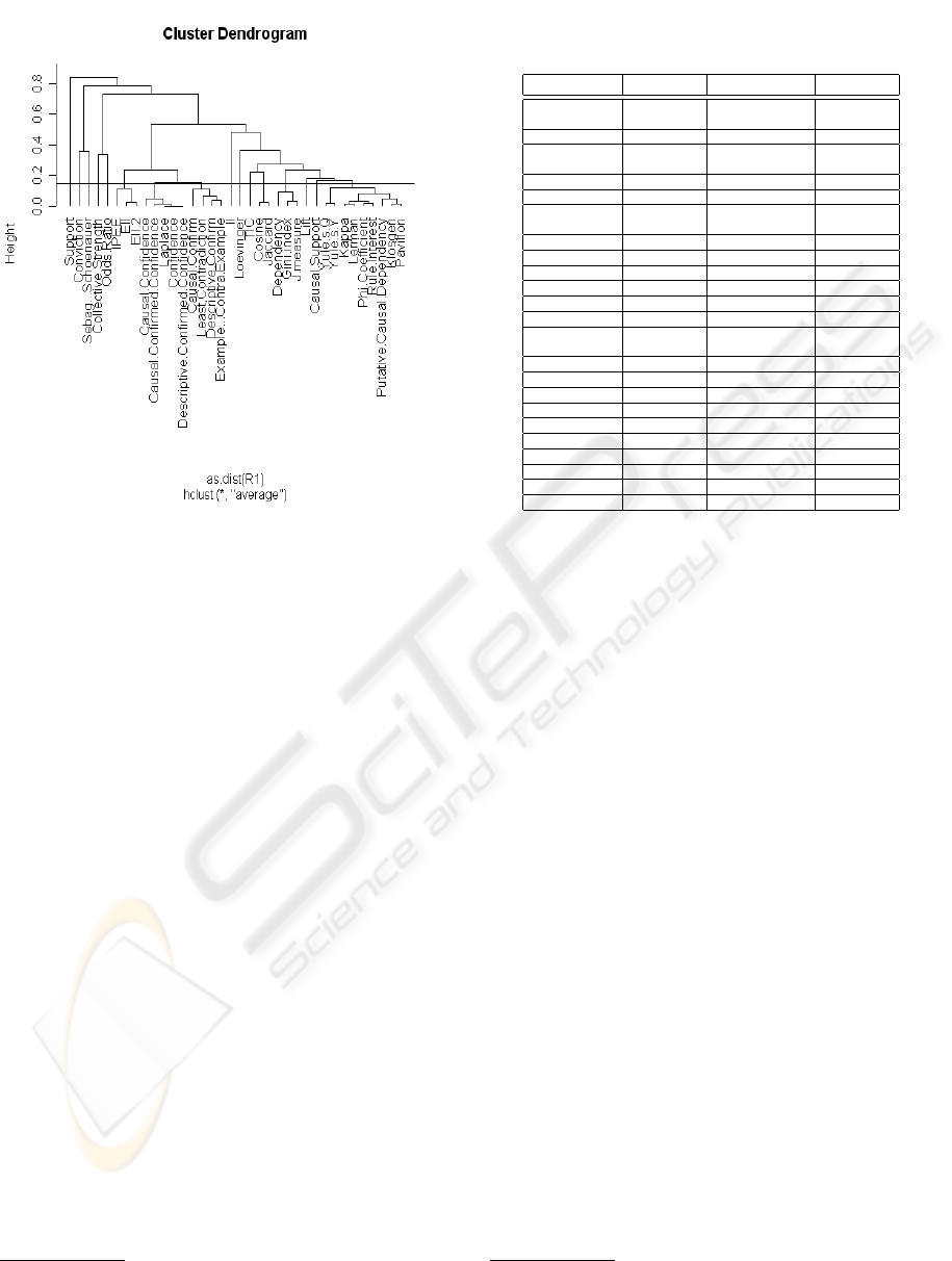
Figure 1: View on the strong relation between IMs.
5.1 View of Strong Relation
The strong relations between IMs are obtained by cut-
ting the dendrogram (AHC) from the bottom with a
small value of dissimilarity d =0.15
1
(see Fig. 1 for
R
1
). The clusters are formed by the hierarchy of IMs
in the zone under the horizontal line. The same result
can be seen in Tab. 3 in which each column represent-
ing for a ruleset.
This view is helpful because the user can choose
the clusters of IMs representing the strong agree-
ment between IMs. In each cluster, a repre-
sented IM can be selected as a representative IM
for all the IMs in the cluster. For example, one
can select Laplace as the representative IM for
the confidence cluster (Causal Confidence, Causal
Confirmed-Confidence, Laplace, Confidence, De-
scriptive Confirmed-Confidence). This cluster is use-
ful to discover the rules having the strong effect of
confidence value.
Tab. 4 illustrates the five comparisons between the
four rulesets (vertically). The first four columns show
the comparison for each pair of rulesets. The last col-
umn illustrates the comparison results obtained from
the four rulesets.
1
The value ρ =0.85 is used because of its widely ac-
ceptable in the literature.
Table 3: Clusters of IMs with the strong relations (IMs rep-
resented by their orders).
R
1
R

1
R
2
R

2
0,2,5,10,21 0,2,5,10,21 0,2,5,8,10,11,12, 0,2,5,8,10,
16,21,25,27,29 21,25,27,29
1,9,13,22 1,9,13,22 1,9 1,9
3 3,19,20,23, 3 3
24,27,28,30
4 4 4 4,32
6 6 6,31 6,31
7,17 7,17 7,17,19,23,28 7,17,19,23,
28,30,34,35
8,14,18 8,14,18
11,12,16 11,12 11,12,16
13 13
14,18 14,18,20
15 15 15,34,35 15
16
19,20,23,27,
28,29,30,34,35
20
22 22
24 24 24,26
25 25,29
26 26 26
30
31 31
32 32 32
33 33 33 33
34,35
5.2 View of Relative Distance
Consider the number of clusters calculated from the
precedent view, we can apply the PAM method to see
the relative distance
2
between IMs. Fig. 2 illustrates
the clusters of IMs in ellipse shape. The number rep-
resents the cluster order and each cluster has its spe-
cific symbol.
The complementary information obtained from the
clusters in this view is useful to the user. By observ-
ing the diameter (smallest, biggest, ...) or the other
parameters (separation, maximum distance, minimum
distance, ...) one can choose the clusters to examine
as different aspects from the dataset, each cluster is
then represented by a representative IM. This repre-
sentative IM is calculated as a medoid in the cluster.
For example in Fig. 2, Tab. 5, cluster 2 (Least Con-
tradiction, Example & Contra-Example, Causal Con-
firm, Descriptive Confirm) one can have Example &
Contra-Example as the representative IM having the
strong effect of negative examples.
Tab. 6, the same way to compare the results be-
tween rulesets as Tab. 4, gives all common clusters
obtained from the four rulesets evaluated. At the fifth
column, we can see an interesting cluster with only
one IM : TIC (33), is the original IM for capturing an
aspect of informational ratio modulated by the contra-
positive.
2
By using the PCA (Principal Component Analysis)
technique.
DISCOVERING THE STABLE CLUSTERS BETWEEN INTERESTINGNESS MEASURES
199

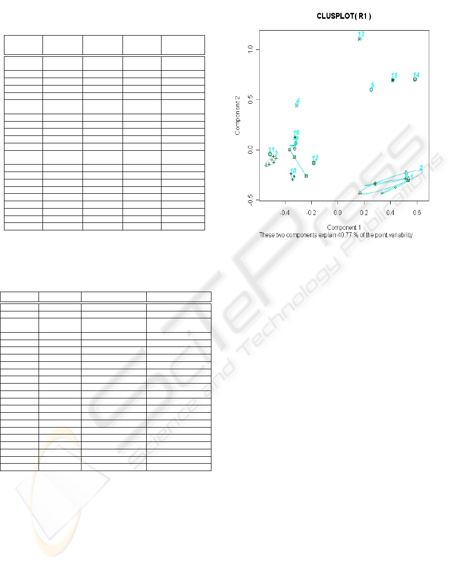
Table 4: Cluster comparison from the strong relation view
(IMs represented by their orders).
R
1
∩ R

1
R
2
∩ R

2
R

1
∩ R

2
R
1
∩ R
2
R
1
∩ R

1
∩
R
2
∩ R

2
0,2,5,10,21 0,2,5,8,10, 0,2,5,10,21 0,2,5,10,21 0,2,5,10,21
21,25,27,29
1,9,13,22 1,9 1,9 1,9 1,9
3 3
4 4
6 6,31
7,17 7,17,19, 7,17 7,17 7,17
23,28
8,14,18
11,12 11,12,16 11,12 11,12,16 11,12
13
14,18 14,18 14,18 14,18
15 15
19,20,23, 19,23,28,30 19,23,28 19,23,28
27,28,30
22
24
25,29
26 26
27,29
31
32 32
33 33 33 33 33
34,35 34,35 34,35 34,35 34,35
Table 5: Clusters of IMs with the relative distance (IMs rep-
resented by their orders).
R
1
R

1
R
2
R

2
0,2,5,10,21 0,1,2,5,10,21 0,2,5,8,10,21,25,27,29 0,2,5,8,10,21,25,27,29
1,9,13,22 1,9 1,9
3,19,23,28, 3,19,20,23, 3 3
30,34,35 24,27,28,30
4 4 4 4,14,18,20
6 6 6,31 6,31
7,17 7,17 7,17,19,23,28 7,17,19,23,28,30
8,14,18 8,14,18
9,13,22
11,12,16 11,12 11,12,16 11,12,16
13 13
14,18,30
15 15 15,34,35 15,34,35
16
20,27,29 20
22 22
24 24 24,26
25 25,29
26 26 26
31 31
32 32 32 32
33 33 33 33
34,35
5.3 Stable Clusters
From the two different evaluations based on the two
views of strong relation and relative distance, the
more surprising result appears. By analyzing the fifth
column from Tab. 4 and Tab. 6, eight stable clusters
are found indicating an invariance with the nature of
the dataset!.
- The first cluster (Causal Confirmed-Confidence,
Laplace, Confidence, Descriptive Confirmed-
Confidence, Causal Confidence) has most of the
Figure 2: Views on the relative distance between clusters of
IMs.
measures issued from the Confidence measure.
- The second cluster (Cosine, Jaccard) has a strong
relation with the fifth property proposed by Tan et al.
(Tan et al., 2004).
- The third cluster (EII 2, EII) are two measures ob-
tained with different parameters of the same original
formula and very useful in evaluating the entropy of
implication intensity.
- The fourth cluster (Gini-index, J-measure) is an
entropy cluster.
- The fifth cluster (Kappa, Lerman, Phi-
Coefficient) is a set of similarity IMs.
- The sixth cluster (Support) indicates the influence
of the support values of the rule.
- The seventh cluster (TIC) has only one measure
provides the strong evaluation on the information ra-
tio modulated by contrapositive.
- The last cluster (Yule’s Y, Yule’s Q) gives triv-
ial observation because the measures are all derived
from Odds Ratio measure, that is similar to the second
property proposed by Tan et al. (Tan et al., 2004).
6 CONCLUSION
Discovering the behaviors of IMs is an interesting re-
search and with the obtained results we can strongly
help the user understand different hidden aspects ex-
isting on specific datasets. The evaluation of various
IMs on the datasets having opposite characteristics is
ICEIS 2006 - ARTIFICIAL INTELLIGENCE AND DECISION SUPPORT SYSTEMS
200

Table 6: Cluster comparison from the relative distance view
(IMs represented by their orders).
R
1
∩ R

1
R
2
∩ R

2
R

1
∩ R

2
R
1
∩ R
2
R
1
∩ R

1
∩
R
2
∩ R

2
0,2,5,10,21 0,2,5,8,10, 0,2,5,10,21 0,2,5,10,21 0,2,5,10,21
21,25,27,29
1,9 1,9
3,19,23, 3
28,30
4 4
6 6,31
7,17 7,17,19,23,28 7,17 7,17 7,17
8,14,18
9,13,22
11,12 11,12,16 11,12 11,12,16 11,12
13
14,18 14,18 14,18 14,18
15 15,34,35
19,23,28,30 19,23,28 19,23,28
20,27
22
24
25,29
26 26
27,29
31
32 32 32 32 32
33 33 33 33 33
34,35 34,35 34,35 34,35
an important method. By calculating the dissimilar-
ity between 36 IMs, we have determined eight stable
clusters of IMs as eight different aspects found from
the two opposite datasets.
The eight stable clusters denote an interesting re-
lations between IMs because they remark the stable
behaviors.
REFERENCES
Agrawal, R., Mannila, H., Srikant, R., Toivonen, H., and
Verkano, A. (1996). Fast discovery of association
rules. In Advances in Knowledge Discovery in Data-
bases. AAAI/MIT Press.
Blanchard, J., Guillet, F., Gras, R., and Briand, H.
(2005a). Assessing rule interestingness with a prob-
abilistic measure of deviation from equilibrium. In
ASMDA’05, Proceedings of the 11th International
Symposium on Applied Stochastic Models and Data
Analysis.
Blanchard, J., Guillet, F., Gras, R., and Briand, H. (2005b).
Using information-theoretic measures to assess asso-
ciation rule interestingness. In ICDM’05, Proceed-
ings of the 5th IEEE International Conference on Data
Mining.
Blanchard, J., Kuntz, P., Guillet, F., and Gras, R. (2003).
Implication intensity: from the basic statistical defin-
ition to the entropic version (Chap. 28). In Statistical
Data Mining and Knowledge Discovery.
Carvalho, D. R., Freitas, A. A., and Ebecken, N. F. F.
(2003). A critical review of rule surprisingness mea-
sures. In Proceedings of Data Mining IV - Interna-
tional Confeference on Data Mining.
Carvalho, D. R., Freitas, A. A., and Ebecken, N. F. F.
(2005). Evaluating the correlation between objective
rule interestingness measures and real human interest.
In PKDD’05, the 9th European Conference on Prin-
ciples and Practice of Knowledge Discovery in Data-
bases.
Choi, D. H., Ahn, B. S., and Kim, S. H. (2005). Priori-
tization of association rules in data mining: Multiple
criteria decision approach. In ESA’05, Expert Sytems
with Applications.
Freitas, A. (1999). On rule interestingness measures. In
Knowledge-Based Systems, 12(5-6). Elsevier.
Gavrilov, M., Anguelov, D., Indyk, P., and Motwani, R.
(2000). Mining the stock market: which measure is
best? In KDD’00, Proceedings of the 6th Interna-
tional Conference on Knowledge Discovery and Data
Mining.
Gras, R., Briand, H., Peter, P., and Philipp
´
e, J. (1996). Im-
plicative statistical analysis. In IFCS’96, Proceedings
of the Fifth Conference of the International Federation
of Classification Societies. Springer-Verlag.
Hilderman, R. and Hamilton, H. (2001). Knowledge Dis-
covery and Measures of Interestingness. Kluwer Aca-
demic Publishers.
Huynh, X.-H., Guillet, F., and Briand, H. (2005). Clustering
interestingness measures with positive correlation. In
ICEIS’05, Proceedings of the 7th International Con-
ference on Enterprise Information Systems.
Kaufman, L. and Rousseeuw, P. (1990). Finding Groups in
Data: An Introduction to Cluster Analysis. Wiley.
Kl
¨
osgen, W. (1996). Explora: a multipattern and multistrat-
egy discovery assistant. In Advances in Knowledge
Discovery and Data Mining. AAAI/MIT Press.
Major, J. and Magano, J. (1995). Selecting among rules
induced from a hurricane database. In Journal of In-
telligent Information Systems 4(1).
Newman, D., Hettich, S., Blake, C., and Merz, C. (1998).
[UCI] Repository of machine learning databases,
http://www.ics.uci.edu/∼mlearn/MLRepository.html.
University of California, Irvine, Dept. of Information
and Computer Sciences.
Piatetsky-Shapiro, G. (1991). Discovery, analysis and pre-
sentation of strong rules. In Knowledge Discovery in
Databases. MIT Press.
Ross, S. (1987). Introduction to probability and statistics
for engineers and scientists. Wiley.
Tan, P.-N., Kumar, V., and Srivastava, J. (2004). Selecting
the right objective measure for association analysis. In
Information Systems 29(4). Elsevier.
DISCOVERING THE STABLE CLUSTERS BETWEEN INTERESTINGNESS MEASURES
201