
BENEFICIAL SEQUENTIAL COMBINATION OF
DATA MINING ALGORITHMS
Mathias Goller
Department of Business Informatics - Data & Knowledge Engineering, Johannes-Kepler-University Linz/Austria
Markus Humer
Michael Schrefl
Department of Business Informatics - Data & Knowledge Engineering, Johannes-Kepler-University Linz/Austria
Keywords:
Sequences of data mining algorithms, pre-computing intermediate results, clustering, decision tree construc-
tion, naive bayes.
Abstract:
Depending on the goal of an instance of the Knowledge Discovery in Databases (KDD) process, there are
instances that require more than a single data mining algorithm to determine a solution. Sequences of data
mining algorithms offer room for improvement that are yet unexploited.
If it is known that an algorithm is the first of a sequence of algorithms and there will be future runs of other
algorithms, the first algorithm can determine intermediate results that the succeeding algorithms need. The
anteceding algorithm can also determine helpful statistics for succeeding algorithms. As the anteceding algo-
rithm has to scan the data anyway, computing intermediate results happens as a by-product of computing the
anteceding algorithm’s result.
On the one hand, a succeeding algorithm can save time because several steps of that algorithm have already
been pre-computed. On the other hand, additional information about the analysed data can improve the quality
of results such as the accuracy of classification, as demonstrated in experiments with synthetical and real data.
1 INTRODUCTION
Sophisticated algorithms analyse large data sets for
patterns in the data mining phase of the KDD process.
Depending on the goal the analyst is striving for
when performing an analysis, he or she must apply a
combination of data mining algorithms to achieve that
goal.
We observed in a project with NCR Teradata Aus-
tria that the same data is analysed several times—yet,
each time with different purpose. Typically, several
pre-analyses antecede an analysis. In most of these
analyses data mining algorithms are involved.
Clustering is often used to segment a data set
of heterogenous objects into subsets of objects that
are more homogenous than the unsegmented data
set. Succeeding algorithms analyse these homoge-
nous data sets for interesting patterns, for instance to
find some kind of predictive model such as a churn
model that can be used to predict the probability a
customer will cancel one’s contract in a given time
frame. In other words, clustering and classification
algorithms are used in combination to achieve a com-
mon goal—in this case to determine a churn model
per segment.
A company can also use the combination of clus-
tering and classification algorithms to determine seg-
ments that it can easily identify a customer’s segment.
Otherwise, there could be too many customers which
are erroneously assigned to a segment.
When there is a sequence of data mining algo-
rithms analysing data, the conventional way is to com-
pute the results of each algorithm individually. We
will call that kind of sequential computation of a
combination of data mining algorithms na
¨
ıve com-
bined data mining because this proceeding lacks to
exploit potential improvements the combination of al-
gorithms offers.
Figure 1 illustrates (a) the conventional way of
combining data mining algorithms and (b) our im-
proved way of combining algorithms, which is
sketched in the remainder of this section.
In a sequence of algorithms, each algorithm within
that sequence has the role of antecessor or succes-
sor of another algorithm. Although algorithms in the
middle of a sequence with more than two algorithms
can have both roles, there is only one antecessor and
one successor in each pair of algorithms.
The antecessor retrieves tuples and performs some
operations on them such as determining groups of
135
Goller M., Humer M. and Schrefl M. (2006).
BENEFICIAL SEQUENTIAL COMBINATION OF DATA MINING ALGORITHMS.
In Proceedings of the Eighth International Conference on Enterprise Information Systems - AIDSS, pages 135-143
DOI: 10.5220/0002495501350143
Copyright
c
SciTePress

(a) na
¨
ıve combined data mining
Anteceding
Algorithm A
Succeeding
Algorithm S
S processes result of A
(b) antecessor knows successor
Anteceding
Algorithm A
Succeeding
Algorithm S
S processes result of A
antecessor pre-computes
intermediate results and auxiliary data
Figure 1: Conventional and improved way of sequences in
algorithm combinations.
similar tuples or marking some tuples as relevant ac-
cording to a given criterion. The successor needs the
antecessor’s result or the modifications the antecessor
has applied to the data because otherwise both algo-
rithms could have been run in parallel.
In this work we examine only sequences of data
mining algorithms that are connected due to their re-
sults, i.e. the result of one algorithm is needed for an-
other algorithm. Thus, parallelising unconnected data
mining algorithms is no issue of this work.
If it is known that there will be a run of the suc-
cessor, the antecessor can do more than processing its
own task: During a scan of the data the antecessor
can compute intermediate results the successor needs
and auxiliary data the successor can profit of. As ac-
cessing tuples on a hard disk takes much more time
than CPU operations do, additional computations are
almost for free once a tuple is loaded into main mem-
ory.
Profiting of intermediate results and auxiliary data
means that the succeeding algorithm is either faster or
it returns results of higher quality than in the case of
not-using intermediate results and auxiliary data.
We call the approach of the antecessor preprocess-
ing items for the successor antecessor knows succes-
sor because the task of the successor must be known
when starting the antecessor.
We demonstrate in a series of experiments that the
approach antecessor knows successor is beneficial for
succeeding data mining algorithms. As some results
have been declared as corporate secret by our indus-
trial partner only half of our tests shown in this paper
are made with real data. Where free real data was un-
available we re-did tests with synthetical data having
similar characteristics.
The remainder of this paper is organised as follows:
Section 2 discusses related work in literature. Previ-
ous work concentrates on what we refer to as na
¨
ıve
combined data mining . Section 3 describes how an
anteceding algorithm can pre-compute intermediate
results for later usage by succeeding algorithms. The
experimental results section, section 4, discusses the
results of our experiments based on costs and benefits
of our approach. It also concludes this paper.
2 RELATED WORK
This section surveys previous work on using combi-
nations of data mining algorithms. Previous work can
be classified in (a) work on solving a complex prob-
lem of knowledge discovery by combining a set of
algorithms of different type and (b) work on solving a
problem by using a combination of algorithms of the
same type.
Our discussion of previous work below shows that
especially combining algorithms of different type of-
fers much room for improvement.
2.1 Using Different Types of Data
Mining Algorithms to Solve
Complex Problems
The combination of clustering and classification is the
by far most used combination of different types of
data mining algorithms we found in literature. Hence,
this paper focusses on the combination of clustering
and classification. However, we also present how to
apply our concept on other combinations in short be-
cause the concept is not limited to clustering and clas-
sification.
Several approaches like (Kim et al., 2004) and
(Genther and Glesner, 1994) use clustering to im-
prove the accuracy of a succeeding classification al-
gorithm when there are too many different attributes
for classification. Having less attributes is desirable
because there are less combinations of attributes pos-
sible. As a consequence of less combinations, the re-
sulting trees are less vulnerable to over-fitting.
Approaches of text classification such as (Dhillon
et al., 2002) pre-cluster words in groups of words be-
fore predicting the category of a document. Again, the
accuracy of classification rises due to the decreasing
number of different words.
However, all above-mentioned approaches com-
bine clustering and classification without taking po-
tential improvements in the algorithms. The algo-
rithms are merely executed sequentially. Hence, we
call such approaches na
¨
ıve combined data mining.
Combinations of association rule analysis (ARA)
and other data mining techniques include the com-
binations clustering succeeded by ARA, classification
succeeded by ARA, and ARA succeeded by clustering.
ICEIS 2006 - ARTIFICIAL INTELLIGENCE AND DECISION SUPPORT SYSTEMS
136

There exist several approaches that reduce the num-
ber of found rules by clustering such as (Lent et al.,
1997) and (Han et al., 1997). Unfortunately, the
herein presented auxiliary data are unable to improve
approaches of this kind. Thus, we omit this combina-
tion in further sections.
In web usage mining, an anteceding clustering of
web sessions partitions user in groups having a dif-
ferent profile of accessing a web site. A succeeding
association rule analysis examines patterns of naviga-
tion segment by segment, as shown in (Lai and Yang,
2000) or (Cooley, 2000). However, most papers focus
on either ARA or clustering, as shown in (Facca and
Lanzi, 2005).
Again in web usage mining, a classification algo-
rithm can determine filter rules to distinguish accesses
of human users and software agents which is needed
as only user accesses represent user behaviour.
Both, a clustering algorithm and the scoring func-
tion of a classification algorithm, scan all data the suc-
ceeding ARA algorithm needs. Thus, they could effi-
ciently pre-compute intermediate results for an asso-
ciation rule analysis.
However, all above-mentioned approaches are ap-
proaches of na
¨
ıve combined data mining. Hence, they
are candidates for being improved by our approach as
shown in section 3.
There are data mining algorithms such as the ap-
proaches of (Kruengkrai and Jaruskulchai, 2002) and
(Liu et al., 2000) that call other data mining algo-
rithms during their run. Hereby, there is a strong
coupling between both algorithms as the calling algo-
rithm cannot exist on its own. The calling algorithm
would become a different algorithm when removing
the call of the other algorithm. Thus, we do not call
this coupling of algorithms a sequence of algorithms
because one cannot separate them. In contrast to that
our approach uses loosely coupled algorithms where
each algorithm can exist on its own.
2.2 Combining Data Mining
Algorithms of the Same Type to
Improve Results
Combining data mining algorithms of the same type
to solve a problem is a good choice when there is a
trade-off between speed and quality. Fast but inac-
curate algorithms find initial solutions for succeeding
algorithms that deliver better results but need more
time. k-means (MacQueen, 1967) and EM (Demp-
ster et al., 1977) is such a combination where k-means
generates an initial solution for EM.
Some approaches that cluster streams use hierar-
chical clustering to compress the data in a dendro-
gram which a partitioning clustering algorithm uses
as a replacement of tuples. Using this combination,
only one scan of data is needed—which is a necessary
condition to apply an algorithm on a data stream. Par-
titioning clustering algorithms typically need multiple
scans of the data they analyse. (O’Callaghan et al.,
2002), (Guha et al., 2003), (Zhang et al., 2003), and
(Chiu et al., 2001) are approaches that use a dendro-
gram to compute a partitioning clustering.
An algorithm clustering streams must scan the data
at least once. Thus, algorithms clustering data streams
need a scan in any case.
As the above-mentioned approaches of clustering
streams need only the minimum number of scans,
there is not much room for improvement. (Bradley
et al., 1998) have shown that quality of clustering re-
mains high when using aggregated representations of
data such as a dendrogram instead of the data itself.
Thus, the approaches clustering streams mentioned
above are not limited to streams.
As combining clustering algorithms of the same
type is established in research community, the herein-
presented approach focusses on combinations of data
mining algorithms of different type.
3 ANTECESSOR KNOWS
SUCCESSOR
This section describes the concept antecessor knows
successor in detail. It is organised as follows: Sub-
section 3.1 introduces different types of intermediate
results and auxiliary data. Subsection 3.2 shows their
efficient computation during the antecessor’s run. The
subsequent subsections describe the beneficial usage
of intermediate results and auxiliary data in runs of
succeeding algorithms that are association rule algo-
rithms in subsection 3.3, decision tree algorithms in
subsection 3.4, and na
¨
ıve bayes classification algo-
rithms in subsection 3.5.
3.1 Intermediate Results and
Auxiliary Data
The antecessor can compute intermediate results or
auxiliary data for the successor.
We call an item an intermediate result for the suc-
cessor if the successor would have to compute that
item during its run if not already computed by the an-
tecessor.
Further, we call a date an auxiliary date for the suc-
cessor if that item is unnecessary for the successor to
compute its result but either improves the quality of
the result or simplifies the successor’s computation.
Therefore, the type of the succeeding algorithm de-
termines whether an item is an intermediate result or
BENEFICIAL SEQUENTIAL COMBINATION OF DATA MINING ALGORITHMS
137

an auxiliary date. An item can be intermediate re-
sult in the one application and an auxiliary date in the
other one. For instance, statistics of the distribution of
tuples are intermediate results for na
¨
ıve Bayes classi-
fication but are auxiliary data for decision tree classi-
fication.
Both, intermediate results and auxiliary data, are
either tuples fulfilling some special condition or some
statistics of the data. For instance, tuples that are
modus, medoid, or outliers of the data set are tuples
fulfilling a special condition—modus and medoid
represent typical items of the data set, while outliers
represent atypical items. Furthermore, all kind of sta-
tistics such as mean and deviation parameter are po-
tential characteristics of the data.
We call a tuple fulfilling a special condition an aux-
iliary tuple while we denote an additionally computed
statistic of the data an auxiliary statistic.
3.2 Requirements for Efficient
Computation of Intermediate
Results and Auxiliary Data
This section shows what is required to efficiently
compute intermediate results and auxiliary data for
the successor. It concentrates on the cost of com-
puting and storing intermediate results and auxiliary
data. Their beneficial usage depends on the type of
the succeeding algorithm. Hence, the description of
using intermediate results and auxiliary data is part of
the following subsections 3.3, 3.4, and 3.5.
For computing the antecessor’s result, intermedi-
ate results and auxiliary data in parallel, it must be
possible to compute intermediate results and auxiliary
data without additional scans of the data. Otherwise,
pre-computing intermediate results and auxiliary data
would decrease the antecessor’s performance without
guaranteeing that the successor’s performance gain
exceeds the successor’s performance loss. Conse-
quentially, our approach is limited to auxiliary data
and intermediate results that can easily be determined.
Statistics such as mean and deviation are easy to
compute as count, linear sum, and sum of squares of
tuples is all that is needed to determine mean and de-
viation.
Hence, count, linear sum and sum of squares are
easily-computed items that enable the computation of
several auxiliary statistics.
If the antecessor is a clustering algorithm, auxil-
iary statistics can be statistics of a cluster or statistics
of all tuples of the data set. As the number of clus-
ters of a partitioning clustering algorithm is typically
much smaller than the number of tuples, storing auxil-
iary statistics of all clusters is inexpensive. Thus, we
suggest to store all of them. Our experiments show
that cluster-specific statistics enable finding good split
points when the successor is a decision tree algorithm.
Other statistics like the frequencies of attribute val-
ues and the frequencies of the k most frequent pairs
of attribute values are also easy to compute as shown
in subsections 3.3 and 3.5, respectively.
The cost of determining whether a tuple is an aux-
iliary tuple or not depends on the special condition
which that tuple must fulfill. The mode of a data set
is easy to determine. However, determining if a tuple
is an outlier or a typical representative of the data set
is difficult because one requires the tuple’s vicinity to
test the conditions “is outlier” and “is typical repre-
sentative”. Tuples in sparse areas are candidates for
outliers. In analogy to that, tuples in dense areas are
candidates for typical representatives.
However, if the anteceding algorithm is an itera-
tively optimising clustering algorithm such as EM or
k-means, the task of determining whether a tuple is
a typical representative or an outlier simplifies to the
task of determining whether the tuple is within the
vicinity of the cluster’s centre, or far away of its clus-
ter’s centre.
Further, intermediate results must be independent
of any of the successor’s parameters because the spe-
cific value of a parameter of the successor might be
unknown when starting the antecessor. For instance,
it could be known there will be a succeeding classi-
fication but the analyst has not yet specified which
attribute will be the class attribute.
Yet, if a parameter of the successor has a domain
with a finite number of distinct values, the succes-
sor can pre-compute intermediate results for all po-
tential values of this parameter. For instance, assume
that the class attribute is unknown. Then, the class at-
tribute must be one of the data set’s attributes. To be
more specific, it must be one of the ordinal or categor-
ical attributes that are non-unique, as shown in section
4.2.2. Section 4.2.2 also shows that small buffers are
sufficient to store auxiliary statistics for all potential
class attributes.
3.3 Intermediate Results for
Association Rule Analyses
If the succeeding algorithm is an algorithm which
mines association rules such as apriori or FP-growth,
the frequency of all item sets with one element is
a parameter-independent intermediate result: Apriori
(Agrawal and Srikant, 1994) can then determine the
frequent item sets of length 1 without scanning the
data. FP-growth (Han et al., 2000) can also then de-
termine the item to start the FP-tree with—which is
the most-frequent item—without scanning the data.
Therefore having pre-computed the frequencies of
1-itemsets as intermediate results during the anteces-
ICEIS 2006 - ARTIFICIAL INTELLIGENCE AND DECISION SUPPORT SYSTEMS
138

sor’s run saves exactly one scan. If the additional time
is less than the time of a scan, we receive an improve-
ment in runtime.
As the saving is constantly a scan and the results are
identical with or without pre-computed frequencies,
we omit presenting tests in the experimental results
section.
If it is known which attribute represents the item of
the succeeding association rule analysis, the anteces-
sor can limit the number of potential 1-itemsets. Oth-
erwise, the antecessor must compute the frequency of
each attribute value for all ordinal and categorical at-
tributes.
Even for large numbers of attributes and different
attribute values per attribute, the space that is nec-
essary to store the frequency of 1-itemsets is small
enough to easily fit in the main memory of an up-
to-date computer. We exclude attributes with unique
values because they would significantly increase the
number of 1-itemsets while using them in an associa-
tion rule analysis makes no sense.
3.4 Auxiliary Data for Decision Tree
Classification
Classification algorithms generating decision trees
take a set of tuples where the class is known—the
training set—to derive a tree where each path in the
tree reflects a series of decisions and an assignment to
a class. A decision tree algorithm iteratively identifies
a split criterion using a single attribute and splits the
training set in disjoint subsets according to the split
criterion. For doing this, the algorithm tries to split
the training set according to each attribute and finally
uses that attribute for splitting that partitions the train-
ing set best to some kind of metric such as entropy
loss.
Composing the training set and the way the training
set is split influence the quality of the decision tree.
One can choose the training set randomly or one
can choose tuples that fulfill a special condition as el-
ements of the training set. Our experiments in sub-
section 4.2.1 show that accuracy of classification in-
creases when choosing tuples fulfilling a special con-
dition.
Splitting ordinal or continuous attributes is typi-
cally a binary split at a split point: Initially, the al-
gorithm determines a split point. Then, tuples with an
attribute value of the split attribute that is less than the
split point become part of the one subset, tuples with
greater values become part of the other subset.
Determining the split point is non-trivial if the split
attribute is continuous because the number of poten-
tial split points is unlimited.
However, auxiliary statistics describing the distrib-
ution of attributes simplify finding good split points.
Assume that the anteceding algorithm is a partition-
ing clustering algorithm. Thus, the set of auxiliary
statistics also includes a set of statistics of each clus-
ter.
With the auxiliary statistics of each cluster one can
determine a set of density functions for each continu-
ous attribute the decision tree algorithm wants to test
for splitting.
The experiments in section 4.2.1 show that the
points of intersection of all pairs of density functions
are good candidates of split points.
3.5 Intermediate Results and
Auxiliary Data for Naive Bayes
Classification
It is very easy to deduce a naive Bayes-classifier us-
ing only pre-computed frequencies. A naive Bayes-
classifier classifies a tuple t =(t
1
,...,t
d
) as the class
c ∈ C of a set of classes C that has the highest pos-
terior probability P (c|t). The naive Bayes-classifier
needs the prior probabilities P (t
i
|c) and the proba-
bility P (c) of class c—which the successor can pre-
compute—to determine the posterior probabilities ac-
cording to the formula
P (c|t)=P (c)
d
i=1
P (t
i
|c). (1)
Determining the probabilities on the right hand side
of formula 1 requires the number of tuples, the total
frequency of each attribute value of the class attribute,
and the total frequencies of pairs of attribute values
where one element of a pair is an attribute value of the
class attribute, as the probabilities P (c) and P (t
i
|c)
are approximated by the total frequencies F (c) and
F (c ∩ t
i
) as P (c)=
F (c)
n
and P (t
i
|c)=
F (c∩t
i
)
F (c)
,
respectively.
Frequency F (c) is also the frequency of the 1-
itemset {c}, which is an intermediate result stored for
an association rule analysis, as shown in subsection
3.3. As count n is the sum of all frequencies of the
class attribute, the frequency of pairs of attribute val-
ues is the only remaining item to determine.
Storing all potential combinations of attribute val-
ues is very expensive when there is a reasonable num-
ber of attributes but storing the top frequent combina-
tions is tolerable. As the Bayes classifier assigns a
tuple to the class that maximises posterior probabil-
ity, a class with infrequent combinations is rarely the
most likely class because a low frequency in formula
1 influences the product more than several frequen-
cies that represent the maximum probability of 1.
As a potential solution, one can store the top fre-
quent pairs of attribute values in a buffer with fixed
BENEFICIAL SEQUENTIAL COMBINATION OF DATA MINING ALGORITHMS
139

size and take the risk of having a small fraction of
unclassified tuples.
Counting the frequency of attribute value pairs is
only appropriate when the attributes to classify are or-
dinal or categorical because continuous attributes po-
tentially have too many distinct attribute values.
If a continuous attribute shall be used for classifi-
cation, the joint probability density function replaces
the probabilities of pairs of attribute values in formula
1.
The parameters necessary to determine the joint
probability density function such as the covariance
matrix are auxiliary statistics for the succeeding
Bayes classification.
Hence, pre-computed frequencies and a set of pre-
computed parameters of probability density function
are all that is needed to derive a na
¨
ıve Bayes classifier.
Subsection 4.2.2 shows that the resulting classifiers
have high quality.
4 EXPERIMENTS
We exemplify our approach with a series of exper-
iments organised in two scenarios: (a) Combining
clustering with decision tree construction and (b)
combining clustering with na
¨
ıve Bayes classification.
k-means clustering is the antecessor in both sce-
narios. It pre-computes statistics and identifies spe-
cific tuples that could potentially be used as interme-
diate results and auxiliary data as mentioned in sub-
section 3.2. All intermediate results and auxiliary data
needed by the successors in scenarios (a) and (b) are
a subset of these items. We examine the costs for pre-
computing all items.
In scenario (a) we adapt the classification algorithm
Rainforest (Gehrke et al., 2000) to use auxiliary data
consisting of auxiliary tuples and statistics. We inves-
tigate the improvement on classification accuracy by
using these auxiliary data.
In scenario (b) we construct na
¨
ıve Bayes classifiers
using only pre-computed intermediate results consist-
ing of frequent pairs of attribute values. We compare
the classification accuracy using these pre-computed
intermediate results with the conventional way to
train a na
¨
ıve Bayes classifier.
4.1 Cost of Anticipatory
Computation of Intermediate
Results and Auxiliary Data for
the Succeeding Algorithm
The cost of computing intermediate results and aux-
iliary data are two-fold. On the one hand, storing in-
termediate results and auxiliary data requires space.
Table 1: Computational cost of k-means with and without
pre-computing auxiliary data and intermediate results.
time in seconds overhead
tuples
iterations without with in percent
100’000 4 655 710 8
200’000
3 676 780 15
300’000
7 2’123 2’144 1
400’000
3 1’266 1’500 18
500’000
4 1’654 2’064 25
600’000
6 2’636 3’296 25
700’000
6 2’968 3’740 26
800’000
5 3’137 3’720 19
900’000
5 3’506 4’284 22
1’000’000
2 2’297 2’928 27
2’000’000
6 8’492 10’352 22
3’000’000
2 6’209 6’999 13
4’000’000
5 13’745 16’824 22
5’000’000
5 18’925 22’165 17
This space should fit into the main memory to avoid
additional write and read accesses to the hard disk—
which would slow down the performance of computa-
tion. On the other hand, additional computations need
time regardless there are additional disk accesses or
not.
Table 1 shows the cost of runtime of k-means with-
out and with pre-computing intermediate results and
auxiliary data. The data set used in this table is the
largest data set of our test series. It is the syntheti-
cal data set we used in the test series as described in
section 4.2.1.
In the tests of table 1 we saved intermediate re-
sults and auxiliary data to disk such that we receive
the maximum time of overhead.
Yet, the average percentage of additional time is 20
percent when saving intermediate results and auxil-
iary data. In a third of all tests this additional time is
approximately the same amount of time as needed for
an additional scan.
However, in a majority of cases the additionally
needed time is a minor temporal overhead.
The space that is necessary to store intermediate
results and auxiliary data significantly depends on the
type of data mining algorithm that succeeds the cur-
rent algorithm. Hence, we postpone the costs of space
when we discuss the benefit for different types of data
mining algorithms.
4.2 Benefit of Pre-Computed
Intermediate Results
4.2.1 Benefit for Decision Tree Classification
For demonstrating the benefit of auxiliary data for
decision tree classification we modified the Rainfor-
est classification algorithm to use auxiliary data. The
ICEIS 2006 - ARTIFICIAL INTELLIGENCE AND DECISION SUPPORT SYSTEMS
140

0123456
random set A
near set A
far set A
random set B
near set B
far set B
height of tree
without auxiliary statistics with auxiliary statistics
Figure 2: Height of decision tree.
data set used for testing is a synthetical data set hav-
ing two dozens attributes of mixed type. The class
attribute has five distinct values. Ten percent of the
data is noisy to make the classification task harder.
Additionally, classes overlap.
In a anteceding step we applied k-means to find the
best-fitting partitioning of tuples. We use these par-
titions to select tuples that are typical representatives
and outliers of the data set: We consider tuples that
are near a cluster’s centre as a typical representative.
Analogically, we consider a tuple that is far away of
a cluster’s centre as an outlier. Yet, both are auxiliary
tuples according to our definition in section 3.1. Due
to their distance to their cluster’s centre we call them
near and far.
We tested using both kinds of auxiliary tuples as
training set instead of selecting the training set ran-
domly.
In addition to auxiliary tuples we stored auxiliary
statistics such as mean and deviation of tuples of a
cluster in each dimension.
We used these statistics for determining split points
in a succeeding run of Rainforest. After each run we
compared the results of these tests with the results of
the same tests without using auxiliary statistics.
Compactness of tree and accuracy are the measures
we examined. Compacter trees tend to be more resis-
tant to over-fitting, e.g. (Freitas, 2002, p 49). Hence,
we prefer smaller trees. We measure the height of a
decision tree to indicate its compactness.
Using statistics of distribution for splitting returns
a tree that is lower or at maximum as high as the tree
of the decision tree algorithm that uses no auxiliary
statistics, as indicated in figure 2.
The influence of using auxiliary statistics on accu-
racy is ambiguous, as shown in figure 3. Some tests
show equal or slightly better accuracy, others show
worse accuracy than using no auxiliary statistics.
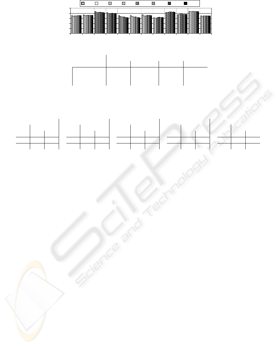
However, using auxiliary tuples as training set sig-
nificantly influences accuracy. Figure 3 shows that
choosing tuples of the near set is superior to choosing
Table 3: Classification accuracy of Bayes classifier with
pre-computed frequencies.
test
S10% S20% S50% aux400 aux1000
accuracy (%) 80.5 81.8 83.5 83.5 83.8
classified (%)
96.6 97.1 98.4 96.9 97.3
total accuracy (%)
77.8 79.4 82.2 80.9 81.2
buffer size 400 1000
pairs of class attribute churn
107 248
tuples randomly.
Considering each test series individually we ob-
serve that the number of tuples only slightly influ-
ences accuracy. Except for the test series foA and
faA, accuracy is approximately constant within a test
series.
Thus, selecting the training set from auxiliary tu-
ples is more beneficial than increasing the number of
tuples in the training set. We suppose that the chance
that there are noisy data in the training set is smaller
when we select less tuples or select tuples out of the
near set.
Summarising, if one is interested in compact and
accurate decision trees then selecting training data out
of the near data set in combination with using statis-
tics about distribution for splitting is a good option.
4.2.2 Benefit for Na
¨
ıve Bayes Classification
For demonstrating the benefit of pre-computing fre-
quencies of frequent combinations for na
¨
ıve Bayes
classification, we compared na
¨
ıve Bayes classifiers
using a buffer of pre-computed frequencies with na
¨
ıve
using the traditional way of determining a na
¨
ıve
Bayes classifier.
We trained na
¨
ıve Bayes classifiers on a real data
set provided by a mobile phone company to us. We
used data with demographical and usage data of mo-
bil phone customers to predict whether a customer is
about to churn or not. Most continuous and ordinal
attributes such as age and sex have few distinct val-
ues. Yet, other attributes such as city have several
hundreds of them. We used all non-unique categori-
cal and ordinal attributes.
For checking the classifiers’ accuracy, we reserved
20 % of available tuples or 9
999 tuples as test data.
Further, we used the remaining tuples to draw sam-
ples of different size and to store the frequencies of
frequent combinations in a buffer.
For storing the top frequent pairs of attribute val-
ues, we reserved a buffer of different sizes. If the
buffer is full when trying to insert a new pair an item
with low frequency is removed from the buffer.
To ensure that a newly inserted element of the list
is not removed at the next insertion, we guarantee a
minimum lifetime t
L
of each element in the list. Thus,
BENEFICIAL SEQUENTIAL COMBINATION OF DATA MINING ALGORITHMS
141
0.0
0.2
0.4
0.6
0.8
1.0
rsoA rsaA noA naA foA faA rsoB rsaB noB naB foB faB
origin of tuples
accuracy
100 200 300 500 1000 2000 3000 5000
tuples in training set
without auxiliary statistics with auxiliary statistics
data set A data set B data set A data set B
random sample rsoA rsoB rsaA rsaB
near tuples noA noB naA naB
legend
far tuples foA foB faA faB
Figure 3: Accuracy of decision tree classifier.
Table 2: Results of Na
¨
ıve Bayes Classification in detail.
sample 10 %
sample 20 % sample 50 % auxiliary buffer 400 auxiliary buffer 1000
actual class
false true
false 7683 1394
estimate
true 487 97
actual class
false true
false 7885 1449
estimate
true 321 52
actual class
false true
false 8195 1494
estimate
true 130 25
actual class
false true
false 8054 1461
estimate
true 140 35
actual class
false true
false 8124 1471
estimate
true 108 31
we remove the least frequent item that has survived at
least t
L
insertions.
Estimating the class of a tuple needs the frequency
of all attribute values of that tuple in combination with
all values of the class attribute. If a frequency is not
present, classification of that tuple is impossible.
A frequency can be unavailable because either (a)
it is not part of the training set or (b) it is not part of
the frequent pairs of the buffer. While option (b) can
be solved by increasing the buffer size, the problem
of option (a) is an immanent problem of Bayes classi-
fication.
Therefore, we used variable buffer sizes and sam-
pling rates in our test series. We tested with a buffer
with space for 400 pairs and 1000 pairs of attribute
values. As the buffer with capacity of 1000 pairs be-
came not full, we left out tests with larger buffers.
Table 3 contains the results of tests with sampling
S10%, S20%, and S50% and results of tests with
buffers as auxiliary data aux400 and aux1000 in sum-
marised form. Table 2 lists these results in detail.
Table 3 shows that small buffers are sufficient for
generating Bayes classifiers with high accuracy.
Although the tests show that classification accuracy
is very good when frequencies of combinations are
kept in the buffer, there are few percent of tuples that
cannot be classified. Thus, we split accuracy in table
3 in accuracy of tuples that could be classified and
accuracy of all tuples. The tests show that the buffer
size influences the number of classified tuples. They
also show that small buffers have a high classification
ratio.
Thus, small buffers are sufficient to generate na
¨
ıve
Bayes classifiers having high total accuracy using ex-
clusively intermediate results.
4.3 Summary of Costs and Benefits
Our experiments have shown that the costs for com-
puting intermediate results and auxiliary data are
low—even, if one saves a broad range of different
types of intermediate results such as the top frequent
attribute value pairs and auxiliary data such as typi-
cal members of clusters to disk. In contrast to that,
the benefit of intermediate results and auxiliary data
is high.
In scenario (a) we examined the effect of using typ-
ical cluster members as auxiliary data on the accu-
racy of a decision tree classification that succeeds a
k-means clustering. We observed that tuples which
are near the clusters’ centres are good candidates of
the training set.
In scenario (b) we examined the accuracy of na
¨
ıve
Bayes classifiers that were generated only by using
frequencies of attribute value pairs calculated as in-
termediate results for the na
¨
ıve Bayes classifier by
an anteceding k-means clustering. These classifiers
had about the same accuracy as conventional classi-
fiers using high sampling rates but could be quickly
computed from the intermediate results.
Furthermore, the general principle of our approach
is widely applicable. For instance, with regards to
ARA we have shown that pre-computing frequencies
of 1-itemsets saves exactly one scan of an association
ICEIS 2006 - ARTIFICIAL INTELLIGENCE AND DECISION SUPPORT SYSTEMS
142

rule analysis without changing the result.
REFERENCES
Agrawal, R. and Srikant, R. (1994). Fast algorithms for
mining association rules. In Bocca, J. B., Jarke, M.,
and Zaniolo, C., editors, Proc. 20th Int. Conf. Very
Large Data Bases, VLDB, pages 487–499. Morgan
Kaufmann.
Bradley, P. S., Fayyad, U. M., and Reina, C. (1998). Scaling
clustering algorithms to large databases. In Knowl-
edge Discovery and Data Mining, pages 9–15.
Chiu, T., Fang, D., Chen, J., Wang, Y., and Jeris, C. (2001).
A robust and scalable clustering algorithm for mixed
type attributes in large database environment. In Pro-
ceedings of the seventh ACM SIGKDD international
conference on Knowledge discovery and data mining,
pages 263–268. ACM Press.
Cooley, R. (2000). Web Usage Mining: Discovery and Ap-
plication of Interesting Patterns from Web Data. PhD
thesis, University of Minnesota.
Dempster, A. P., Laird, N., and Rubin, D. (1977). Maximum
likelihood via the EM algorithm. Journal of the Royal
Statistical Society, (39):1–38.
Dhillon, S. I., Kumar, R., and Mallela, S. (2002). En-
hancded word clustering for hierarchical text classifi-
cation. In Proceedings of the Eighth ACM SIGKDD
International Conference on Knowledge Discovery
and Data Mining, pages 191–200.
Facca, F. M. and Lanzi, P. L. (2005). Mining interesting
knowledge from weblogs: a survey. Data and Knowl-
edge Engineering, 53(3):225–241.
Freitas, A. A. (2002). Data Mining and Knowledge Dis-
covery with Evolutionary Algorithms. Spinger-Verlag,
Berlin.
Gehrke, J., Ramakrishnan, R., and Ganti, V. (2000). Rain-
forest - a framework for fast decision tree construc-
tion of large datasets. Data Mining and Knowledge
Discovery, 4(2/3):127–162.
Genther, H. and Glesner, M. (1994). Automatic generation
of a fuzzy classification system using fuzzy cluster-
ing methods. In SAC ’94: Proceedings of the 1994
ACM symposium on Applied computing, pages 180–
183, New York, NY, USA. ACM Press.
Guha, S., Meyerson, A., Mishra, N., Motwani, R., and
O’Callaghan, L. (2003). Clustering data streams: The-
ory and practice. IEEE Transactions on Knowledge
and Data Engineering, 15.
Han, E.-H., Karypis, G., Kumar, V., and Mobasher, B.
(1997). Clustering based on association rule hyper-
graphs. In Research Issues on Data Mining and
Knowledge Discovery.
Han, J., Pei, J., and Yin, Y. (2000). Mining frequent patterns
without candidate generation. In Chen, W., Naughton,
J., and Bernstein, P. A., editors, 2000 ACM SIGMOD
Intl. Conference on Management of Data, pages 1–12.
ACM Press.
Kim, K. M., Park, J. J., and Song, M. H. (2004). Binary
decision tree using genetic algorithm for recognizing
defect patterns of cold mill strip. In Proc. of the
Canadian Conference on AI 2004, pages 461 – 466.
Springer.
Kruengkrai, C. and Jaruskulchai, C. (2002). A parallel
learning algorithm for text classification. In KDD
’02: Proceedings of the eighth ACM SIGKDD inter-
national conference on Knowledge discovery and data
mining, pages 201–206, New York, NY, USA. ACM
Press.
Lai, H. and Yang, T.-C. (2000). A group-based inference
approach to customized marketing on the web inte-
grating clustering and association rules techniques. In
HICSS ’00: Proceedings of the 33rd Hawaii Interna-
tional Conference on System Sciences-Volume 6, page
6054, Washington, DC, USA. IEEE Computer Soci-
ety.
Lent, B., Swami, A. N., and Widom, J. (1997). Clustering
association rules. In ICDE, pages 220–231.
Liu, B., Xia, Y., and Yu, P. S. (2000). Clustering through
decision tree construction. In CIKM ’00: Proceedings
of the ninth international conference on Information
and knowledge management, pages 20–29, New York,
NY, USA. ACM Press.
MacQueen, J. (1967). Some methods for classification and
multivariate observations. In Proceedings of the 5th
Berkeley Symp. Math. Statist, Prob.
, pages 1:281–297.
O’Callaghan, L., Mishra, N., Meyerson, A., Guha, S., and
Motwani, R. (2002). High-performance clustering of
streams and large data sets. In Proc. of the 2002 Intl.
Conf. on Data Engineering (ICDE 2002), February
2002.
Zhang, D., Gunopulos, D., Tsotras, V. J., and Seeger, B.
(2003). Temporal and spatio-temporal aggregations
over data streams using multiple time granularities.
Inf. Syst., 28(1-2):61–84.
BENEFICIAL SEQUENTIAL COMBINATION OF DATA MINING ALGORITHMS
143
