Clustering by Tree Distance for Parse Tree
Normalisation
Martin Emms
Department of Computer Science, Trinity College, Dublin
Abstract. The application of tree-distance to clustering is considered. Previous
work identified some parameters which favourably affect the use of tree-distance
in question-answering tasks. Some evidence is given that the same parameters
favourably affect the cluster quality. A potential application is in the creation of
systems to carry out transformation of interrogative to indicative sentences, a first
step in a question-answering system. It is argued that the clustering provides a
means to navigate the space of parses assigned to large question sets. A tree-
distance analogue of vector-space notion of centroid is proposed, which derives
from a cluster a kind of pattern tree summarising the cluster.
1 Introduction
In [1] some work was reported on the use of tree-distance in a question-answering task.
Broadly speaking, the aim is to take a parse-structure from a question and match it up
to parse-structures for candidate answers, with variants of approximate tree-matching
algorithms. In this context, it can be desirable to normalise parse structures, applying
transformations to them. One might consider a normalisation of passive structures to
active structures for example, or of interrogative structures, to indicative structures.
Designing such transformations, however, can be a very time consuming task. If
the people writing the transformations are the same people as those that designed the
parser, and its underlying grammatical assumptions, it may be possible to construct the
transformations more or less a priori, from first principles. But that may very well not
be the case. A popular parser is the Collins probabilistic parser [2]. It is trained on
data from the Penn Treebank, and its aim is to produce analyses in its style: indeed
its primary form of testing consists in trying to reproduce a subset of the treebank
which is held out from its training. The trees from the Penn treebank are not assigned
in accordance with any finite grammar. This alone complicates any endeavour to design
a set of transformations from first principles. In addition to that, one is dealing with
the outputs of a probabilistic parser, and its is hard to know ahead of time, how its
particular disambiguation mechanisms will impact on the kind of the trees produced.
Thus, instead of trying to work out the transformations exclusively or even at all from
first principles, one is lead to a situation in which it is necessary to empirically inspect
the trees that the parser generates, and to try to write the transformations a posteriori
after some empirical data exploration. The techniques to be described here are intended
to assist in this phase.
Taking a particular example, suppose there are 500 question sentences (as is typical
in the TREC QA tasks [3]). One would like to design a set of transformations which
Emms M. (2006).
Clustering by Tree Distance for Parse Tree Normalisation.
In Proceedings of the 3rd International Workshop on Natural Language Understanding and Cognitive Science, pages 91-100
DOI: 10.5220/0002502400910100
Copyright
c
 SciTePress

can be applied to the parse structures of these sentences. The simplest possible approach
involves manually looking at each of 500 parse structures, and trying mentally to induce
the generalisations and possible transformations. But with 500 structures that is at the
very least a daunting task
1
. What will be described below is a method by which (i)
the parse structures can be hierarchically clustered by tree-distance and (ii) a kind of
centroid tree for a chosen cluster can be generated which exemplifies the most typical
traits of trees within the cluster.
2 Tree Distance
The tree distance between two trees can be defined by considering all the possible 1-
to-1 partial maps, σ, between source and target trees S and T , which preserve left to
right order and ancestry: if S
i
1
and S
i
2
are mapped to T
j
1
and T
j
2
, then (i) S
i
1
is to
the left of S
i
2
iff T
j
1
is to the left of T
j
2
and (ii) S
i
1
is a descendant of S
i
2
iff T
j
1
is a
descendant of T
j
2
. Nodes of S which are not in the domain of σ are considered deleted,
with an associated cost. Nodes of T which are not in the range of σ are considered
inserted, with an associated cost. Otherwise, where T
j
= σ(S
i
), and T
j
= S
i
, there
is a substitution cost. The least cost belonging to a possible mapping between the trees
defines the tree distance. A simple example is given in the left-hand part of Figure 1.
2.1 Question Answering by Tree Distance
An approach to question answering using tree-distance is described in [1]: potential
answers to a question are ranked according to the their tree-distance from the question.
The concern of [1] and work since then is the variables that influence the performance
of a question-answering system using tree distance. This section will briefly summarise
these findings.
Let a Question Answering by Tree Distance (QATD) task, be defined as a set of
queries, Q, and for each query q, a corpus of potential answer sentences, COR
q
.For
each a ∈COR
q
, the system should determine td(a, q), the tree-distance between a
and q, and use this to sort COR
q
into A
q
. Where a
c
∈A
q
is the correct answer, then
the correct-answer-rank is the rank of a
c
in A
q
: |{a ∈A
q
: td(a, q) ≤ td(a
c
,q)}|
whilst the correct-answer-cutoff is the proportion of A
q
cut off by the correct answer
a
c
: |{a ∈A
q
: td(a, q) ≤ td(a
c
,q)}| / |A
q
|. Note that a QATD task, as a
QA system, is very minimal: with no use made of many techniques which have been
found useful in QA, such as query-expansion, query-type identification, named entity
recognition etc. These are far from being incompatible, but the supposition is that what
is found out about the variables influencing performance on QATD tasks will carry over
to QA system which use tree distance alongside other mechanisms.
One of the aims of syntactic structures is to group items which are semantically
related. But there are many competing aims (such as predicting ellipsis, conformance to
X-bar theory, explaining barriers to movement) with the result that syntactic structures
might encode or represent a great deal that is not semantic in any sense. Following this
1
just looking at each for 5 minutes, will take 41 hours
92

line of thought, on an extremely pessimistic view of the prospects of QATD, it will not
work for any parser, or question/answer set: sorting answers by tree-distance would be
no better than generating a random permutation. On an optimisitic view, at least for
some parsers, and some question/answer sets, the syntactic structures can be taken as an
approximation of semantic structures, and sorting by tree-distance will be useful. For
2 different parsers, and 2 QATD tasks, we have found reasons for the optimistic view,
in the form of the finding that improvements to parse quality lead to improved QATD
performance. The 2 tasks are:
The Library Manual QATD Task: in this case Q is a set of 88 hand-created
queries, and COR
q
, shared by all the queries, is the sentences of the manual of
the GNU C Library
2
.
The TREC 11 QATD task: In this case Q was the 500 questions of the
the TREC11 QA track [3], whose answers are drawn from a large corpus
of newspaper articles. COR
q
was taken to be the sentences of the top 50
from the top-1000 ranking of articles provided by TREC11 for each question
(|COR
q
|≈ 1000). Answer correctness was determined using the TREC11
answer regular expressions
The performance on these QATD tasks has been determined for some variants of
a home-grown parsing system – call it the trinity parser – and the Collins parser [2]
(Model 3 variant). Space precludes giving all the details but the basic finding is that
parse quality does equate to QATD performance. The left-hand data in Table 1 refers
to various reductions of the linguistic knowledge bases of the the trinity parser(thin50
= random removal of 50 % subset, manual = manual removal of a subset, flat = entirely
flat parses, gold = hand-correction of query parses and their correct answers). The right-
hand data in Table 1 refers to experiments in which the repertoire of moves available to
the Collins parser, as defined by its grammar file, was reduced to different sized random
subsets of itself.
Table 1. Distribution of Correct Cutoff across query set Q in different parse settings. Left-hand
data = GNU task, trinity parser, right-hand data = TREC11 task, Collins parser.
Parsing 1st Qu. Median Mean 3rd Qu.
flat 0.1559 0.2459 0.2612 0.3920
manual 0.0215 0.2103 0.2203 0.3926
thin50 0.01418 0.02627 0.157 0.2930
full 0.00389 0.04216 0.1308 0.2198
gold 0.00067 0.0278 0.1087 0.1669
Parsing 1st Qu. Median Mean 3rd Qu.
55 0.3157 0.6123 0.5345 0.766400
75 0.02946 0.1634 0.2701 0.4495
85 0.0266 0.1227 0.2501 0.4380
100 0.01256 0.08306 0.2097 0.2901
The basic notion of tree distance can be varied in many ways, some of which are:
Sub-tree: in this variant, the sub-tree distance is the cost of the least cost mapping from
a sub-tree of the source. Sub-traversal: the least cost mapping from a sub-traversal of
2
www.gnu.org
93

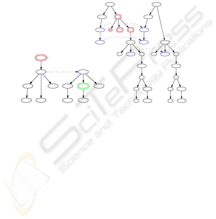
the left-to-right post-order traversal of the source. Structural weights: in this variant
nodes have a weight between 0 and 1, and the weights are assigned according to the
syntactic structure, with adjuncts given 1/5th the weights of heads and complements,
and other daughters 1/2. The righthand alignment in Figure 1 is an example alignment,
where the nodes associated with an auxiliary get a low weight. Wild cards: in this vari-
a
b
b
a
a
c
b
a
b b a
a
p
rocess something
n pro
np
s
vp
rhs
lhs be rhs
lhs
vp
call be
memory
n
n
n
allocation
np
np
s
vp
lhs rhs
memory
n
n
n
allocat
ion
np
Fig.1. (i) an unweighted abstract example (ii) a weighted linguistic example. Deletions shown in
red and double outline, insertions in green and double outline), substitutions in blue and linked
with an arrow; nodes which are mapped unaltered displayed at the same height but with no linking
arrow.
ant, marked target sub-trees can have zero cost matching with sub-trees in the source.
Such wild card trees can be put in the position of the gap in wh-questions, allowing for
example what is memory allocation, to closely match any sentences with memory allo-
cation as their object, no matter what their subject. Lexical Emphasis: in this variant,
leaf nodes have weights which are scaled up in comparision to nodes which are internal
to the tree. String Distance: if you code source and target word sequences as vertical
trees, the string distance [4] between them coincides with the the tree-distance, and the
sub-string distance coincides with the sub-traversal distance.
The impact of these variants on the above-mentioned parsers and QATD tasks has
also been investigated. Table 2 gives the results for the trinity parser on the GNU task
(for the distance type column -we = structural weights, -wi = wild cards, -lex = lexical
emphasis, sub = sub-tree).
94

Table 2. Correct-Answer-Cutoff for different distance measures (GNU task).
distance type 1st Qu. Median Mean
sub-we-wi-lex 9.414e-05 1.522e-03 4.662e-02
substring 2.197e-04 3.609e-03 5.137e-02
sub-we-wi 7.061e-04 1.919e-02 1.119e-01
sub-we 3.891e-03 4.216e-02 1.308e-01
sub 1.517e-02 1.195e-01 1.882e-01
whole 0.040710 0.159600 0.284600
What the data show is that the version of tree distance which uses sub-trees, weights,
wild-cards and lexical emphasis, performs better than the sub-string distance, and that
each of the parameters make a contribution to improved performance.
3 Clustering by Tree Distance
The 500 question sentences of the TREC11 Question Answering task [3] were parsed
using the Collins parser. For any pair of question-structures q
1
, q
2
, the tree-distance,
td(q
1
,q
2
) can be determined, giving a 2 dimensional table of question-to-question dis-
tances. This gives the prerequisites for applying clustering to the set of questions.
We used the agglomerative clustering algorithm [5] as implemented by the R statis-
tical package. This repeatedly picks a pair of clusters out of a larger set of clusters and
merges the pair into a single cluster. The pair of clusters chosen to be merged is the one
minimising an inter-cluster distance measure, defined on top of the point-wise distance
measures, in this work defined to be the average of the point-wise distances:
D(C
1
, C
2
)=(1/ |C
1
|| C
2
|) ×

q
i
∈C
1
,q
j
∈C
2
td(q
i
,q
j
)
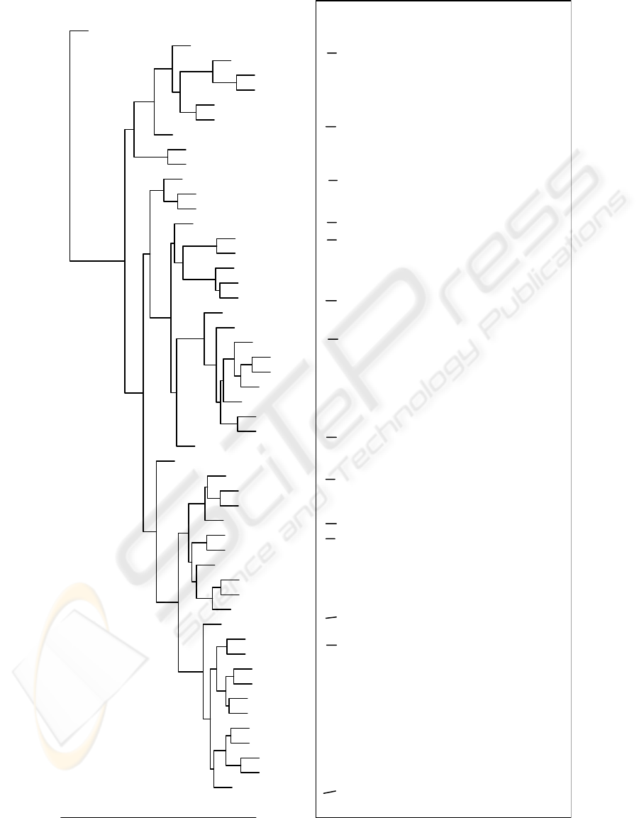
The history of the cluster-merging process can the viewed in a dendogram plot such as
the upper half of figure 2
This example shows the dendogram for the questions which all have who as the
first word
3
. In the lower half of the picture, trees are given which typify the structures
found within a particular cluster. One can see that the clustering gives intuitive results.
For example, numbering the clusters left-to-right, clusters 1-3 all fit the pattern (SBAR
who (S TRACE VP)) – they are trees containing a trace element – whilst clusters
4-7 all fit the pattern (SBARQ who (SQ VB ...)). Then within clusters 1-3 there
is variation within the VP. In cluster 1 you have a verb and a simple NP. In clusters 2
and 3 a PP is involved, either as a part of the VP or as part of the NP.
Even without further automation, such a clustering is useful. One can pick out a
subset of the data and have reasons for thinking that the points in that subset are related:
in the current case, one could have reasons for thinking that all the trees within that
3
Related dendograms were computed for other questions types, such those beginning with what,
which, when etc
95

1891
1772
1712
1686
1563
1746
1457
1643
1640
1535
1479
1431
1780
1678
1428
1759
1610
1424
1724
1670
1440
1602
1805
1890
1822
1476
1733
1573
1426
1412
1464
1538
1769
1835
1716
1622
1788
1553
1395
1777
1533
1598
1863
1511
1821
1817
1782
1664
1475
1417
1589
1494
___SBAR |___who |___S |___TRACE |___VP |___VB |___NP
___SBAR |___who |___S |___TRACE |___VP |___VB |___NP |___PP
___SBAR |___who |___S |___TRACE |___VP |___VB |___NP |___NP |___PP
___SBARQ |___who |___SQ |___VB |___NP |___NP |___PP
___SBARQ |___who |___SQ |___VB |___NP
___SBARQ |___who |___SQ |___VB |___NP |___VP
___SBARQ |___who |___SQ |___VB |___NP |___NP |___SQ |___to |___VP
12
3
4
5
6
7
Fig.2. Dendogram for who questions.
96

cluster might fall within the scope of a particular transformation. Manual inspection
of the suggested subset can then be carried out to see if the tree structures involved
are related in any striking way. Although there is still an element of manual inspection
involved, this could still be an improvement over simply scanning over all the data
points: it will be an improvement when the suggested clusters actually do exhibit some
striking similarity. Working with the TREC questions and the parse structures produced
by the Collins parser we found this to be the case.
There is a number calculated by the agglomerative clustering algorithm – the ag-
glomerative coefficient whose intention is to measure the overall quality of the hierar-
chical clustering produced. For each question q
i
, let S(q
i
) be the first cluster that q
i
is
merged with – its sister in the clustering dendogram. Let merge
dist(q
i
) be the inter-
cluster distance at this merge point for q
i
. Normalising this by the inter-cluster distance
at the last step of the algorithm – call this D
f
– the agglomerative coefficient (AC) is
defined as the average of all 1 − merge
dist(q
i
)/D
f
. This number ranges from 0 to 1,
with numbers closer to 1 interpreted as indicating better clustering [5].
Section 2.1 described previous and ongoing work on using tree distance for question
answering. One finding was that increasing the linguistic knowledge bases available
to the parser, and consequently the sophistication of the parses that the parser is able
to produce, tends to increase the question answering performance. Also structurally
weighting nodes according to a head/complement/adjunct/other distinction gives better
results than weighting all nodes equally. It is interesting to find that the same variations
lead to better values in the quality of clustering, as measured by the agglomerative
coefficient – see Table 3
Table 3. Values of Agglomerative Coefficient for question structure clustering (Collins parser,
TREC11 questions), for different parse settings and different distance measures.
parse setting AC distance setting AC
with weights 55% grammar 0.63 without weights 100% grammar 0.73
with weights 75% grammar 0.75 with weights 100% grammar 0.8
4 Deriving a Pattern Tree from a cluster
Whilst using the clustering can certainly be helpful in navigating the space of analyses,
there is scope for more automation. As a first step, for a given cluster, one can seek the
centre point of that cluster, that point whose average distance to other points is least:
centre(C)=arg
min(q
i
∈C)D({q
i
}, C\{q
i
})
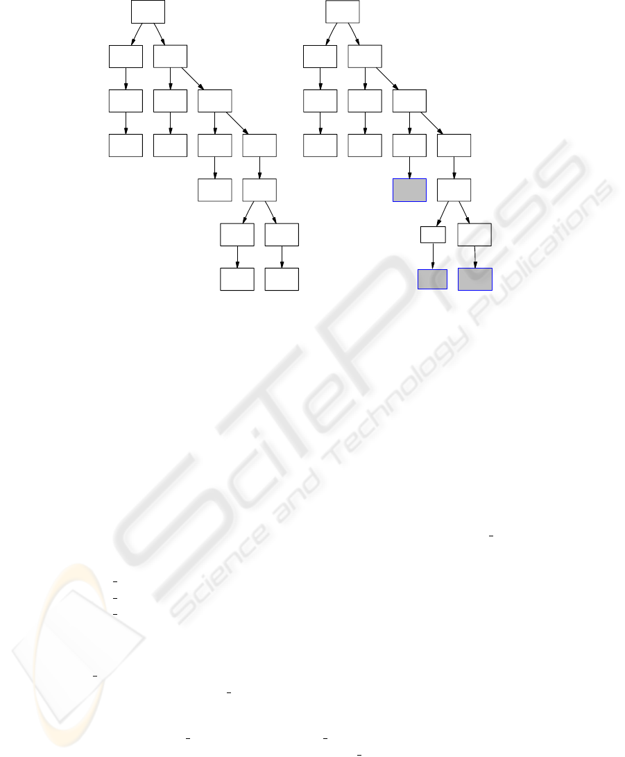
For the first cluster from Figure 2 the most central tree is shown as the lefthand tree in
in Figure 3. While finding this ’most central’ tree centre(C) is some help, one cannot
tell simply by inspection, which parts of the structure are generic, and shared by the
other trees in the cluster, and which are idiosyncratic and not shared. Things which
are idiosyncratric in centre(C) are going to be a distraction if one wishes to take this
central tree as a starting point for describing the target of a transformation.
97

SBAR
WHNP S
WP
Who
TRACE VP
T VB NP
stabbed NPB
NN NN
Monica Seles
SBAR
WHNP S
WP
Who
TRACE VP
T VB NP
stabbed NPB
NN NN
Monica Seles
Fig.3. (i) Central Tree (ii) Alignment Summary from cluster 1 in Fig 2, with typically matched
nodes shown plain, and typically subsituted nodes shown filled.
In many clustering applications, the data points are vectors, with distance defined
by either Euclidean or Cosine distance. In this setting it is typical to derive a centroid
for the cluster, which has in each vector dimension the average of the cluster members’
values on that dimension. The question which naturally presents itself then is
what is the tree-distance analogue of the notion of centroid ?
As far as I am aware, this is not a notion people have looked at before. I want to propose
that a natural way to do this is to refer to the alignments between the computed central
tree, centre(C), and the other trees in C. To that end we define a function align
outcome
such that for each node i in centre(C):
align
outcome(i,0) = number of times node i matched perfectly
align
outcome(i,1) = number of times node i was substituted
align
outcome(i,2) = number of times node i was deleted
Using this we can derive from the central tree an alignment summary tree,
align
sum(C), isomorphic to centre(C), where for each node i ∈ centre(C), there is a
corresponding node i in align sum(C), labelled with an outcome and weighting (o, w)
such that:
o = arg
max(o ∈ 0, 1, 2)(align outcome(i, o))
w = max({w

: o ∈ 0, 1, 2,w

= align outcome(i, o)/ |C|})
98

so each node is annotated with its commonest outcome type and the relative frequency
of that outcome type. Once the display of each node in align
sum(C) has its colour
depend on the outcome type and its size on the weighting, the resulting pictures can
be very helpful in coming up with a pattern for the cluster. Nodes which are typically
matched perfectly are large and black: they are prime candidates to be fixed features
in any pattern for the cluster. Nodes which typically largely substituted are large and
blue (and filled): these are prime candidates to be just wild-cards in any pattern for the
cluster. Nodes which are largely deleted are large and red (and have double outlines):
prime candidates for being missed out from a pattern for the cluster.The righthand tree
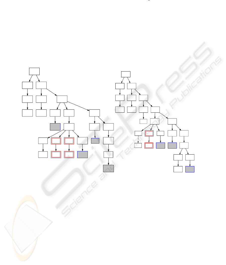
in Figure 3 shows the result of this applied to the central tree shown to the left. Figure 4
shows the results from the second and third clusters from Fig 2.
SBAR
WHNP S
WP
Who
TRACE VP
T VB NP PP
was NPB
DT NN PUN NN
the U.S . president
IN NP
in NPB
NN
1929
SBAR
WHNP S
WP
Who
TRACE VP
T VB NP
was NPB PP
DT JJ NN
the lead singer
IN NP
for NPB
DT NN
the Commod
ore
Fig.4. Alignment Summary trees for clusters 2 and 3 from Fig 2. Typically matched nodes are
plain, typically subsituted nodes shown filled, typically deleted nodes shown red with double
outline.
A final step of automation is to try to automatically derive a pattern from the align-
ment summary tree. To do this red nodes – deletion nodes – are deleted. Subtrees all of
whose nodes are blue – subsitution nodes – are turned into wild-card trees. Doing this
to the 3 examples you get for cluster one:
(SBAR (WHNP WP who)
(S (TRACE T)
(VP (VB
**
V
**
)
(NP (NPB (NN
**
N
**
)(N
**
N
**
))))))
for cluster two:
99

(SBAR (WHNP WP who)
(S (TRACE T)
(VP (VB
**
V
**
)
(NP (DET the) (NN
**
N
**
))
(PP (IN
**
P
**
) (NP (NPB (N
**
N
**
)))))))
for cluster three:
(SBAR (WHNP WP who)
(S (TRACE T)
(VP (VB was)
(NP (NP (NPB (DET the) (NN
**
N
**
)))
(PP (IN
**
P
**
) (NP (NPB (DET the) (N
**
N
**
))))))))
which can serve as starting points for definition of tranformations to turn interroga-
tive who sentences to indicative sentences.
5 Conclusions and Future Work
We have given evidence that adaptations of tree distance which have been found to
improve question answering also seem to improve cluster quality. We have argued that
clustering by tree distance can be very useful in the context of seeking to define transfor-
mations from interrogative to indicative forms, and proposed ways to define an analogue
of cluster centroid for clusters of syntax structures.
Some other researchers have also looked at the use of tree-distance measures in
semantically-oriented tasks [6] [7], using dependency-structures, though, instead of
constituent structures. Clearly the dependency vs constituent structure dimensions needs
to be explored. There are also many possibilities to be explored involving adapting cost
functions, to semantically enriched node descriptions, and to corpus-derived statistics.
One open question is whether analogously to idf, cost functions for (non-lexical) nodes
should depend on tree-bank frequencies.
References
1. Martin Emms. Tree distance in answer retrieval and parser evaluation. In Bernadette Sharp,
editor, Proceedings of NLUCS 2005, 2005.
2. Michael Collins. Head-driven statistical models for natural language parsing. PhD thesis,
University of Pennsylvania, 1999.
3. Ellen Vorhees and Lori Buckland, editors. The Eleventh Text REtrieval Conference (TREC
2002). Department of Commerce, National Institute of Standards and Technology, 2002.
4. V.I.Levenshtein. Binary codes capable of correcting insertions and reversals. Sov. Phys. Dokl,
10:707–710, 1966.
5. L.Kaufman and P.J. Rousseeuw. Finding Groups in Data: An Introduction to Cluster Analysis.
Wiley, 1990.
6. Vasin Punyakanok, Dan Roth, and Wen tau Yih. Natural language inference via dependency
tree mapping: An application to question answering. Computational Linguistics, 2004.
7. Milen Kouylekov and Bernardo Magnini. Recognizing textual entailment with tree edit dis-
tance algorithms. In Ido Dagan, Oren Glickman, and Bernardo Magnini, editors, Pascal Chal-
lenges Workshop on Recognising Textual Entailment, 2005.
100