
STACK ENCODING REVISITED
Yangjun Chen
Dept. Applied Computer Science, University of Winnipeg, Canada
Keywords: XML databases, Trees, Paths, XML pattern matching, Twig joins.
Abstract: The twig join, which is used to find all occurrences of a twig pattern in an XML database, is a core
operation for XML query processing. A great many strategies for handling this problem have been proposed
and can be roughly classified into two groups. The first group decomposes a twig pattern (a small tree) into
a set of binary relationships between pairs of nodes, such as parent-child and ancestor-descendant relations;
and transforms a tree matching problem into a series of simple relation look-ups. The second group
decomposes a twig pattern into a set of paths. Among all this kind of methods, the approach based on the
so-called stack encoding [N. Bruno, N. Koudas, and D. Srivastava, Holistic Twig Hoins: Optimal XML
Pattern Matching, in Proc. SIGMOD Int. Conf. on Management of Data, Madison, Wisconsin, June 2002,
pp. 310-321] is very interesting, which can represent in linear space a potentially exponential (in the number
of query nodes) number of matching paths. However, the available processes for generating such
compressed paths suffer some redundancy and can be significantly improved. In this paper, we analyze this
method and show that the time complexities of path generation in its two main procedures: TwigStack and
TwigStackXB can be reduced from O(m
2
⋅n) to O(m⋅n), where m and n are the sizes of the query tree and
document tree, respectively. Experiments have been done to compare TwigStackXB and ours, which shows
that using our method much less time is needed to generate matching paths.
1 INTRODUCTION
In XML (World Wide Web Consortium, 1991,
2001), data is represented as a tree; associated with
each node of the tree is an element type from a finite
alphabet ∑. The children of a node are ordered from
left to right, and represent the content (i.e., list of
subelements) of that element.
To abstract from existing query languages for
XML, e.g. XPath (World Wide Web Consortium,
1991), XQuery (World Wide Web Consortium,
2001), XML-QL (Deutch and et al, 1999), and Quilt
(Chamberlin and et al, 1999; Chamberlin and et al,
2000), we express queries as tree patterns where
nodes are types from ∑ ∪ {*} (* is a wildcard,
matching any node type) and string values, and
edges are parent-child or ancestor-descendant
relationships. As an example, consider the query tree
shown in Figure 1, which asks for any node of type
b (node 2) that is a child of some node of type a
(node 1). In addition, the b type (node 2) is the
parent of some c type (node 4) and an ancestor of
some d type (node 5). Type b (node 3) can also be
the parent of some e type (node 7). The query
corresponds to the following XPath expression:
a[b[c and //d]]/b[c and e//d].
In Figure 1, there are two kinds of edges: child
edges (c-edges) for parent-child relationships, and
descendant edges (d-edges) for ancestor-descendant
relationships. A c-edge from node v to node u is
denoted by v → u in the text, and represented by a
single arc; u is called a c-child of v. A d-edge is
denoted v ⇒ u in the text, and represented by a
double arc; u is called a d-child of v.
Finding all occurrences of a twig pattern in a
database has been considered as a core operation in
querying tree structured XML data, both in
relational implementation of XML databases, and in
native XML databases.
Recently this problem has received much
attention in database research community and
different strategies have been proposed. Most of
4 c d 5
2 b
d 8
1 a
6 c
b 3
e 7
Figure 1: A query tree.
5
Chen Y. (2007).
STACK ENCODING REVISITED.
In Proceedings of the Third International Conference on Web Information Systems and Technologies - Internet Technology, pages 5-14
DOI: 10.5220/0001260800050014
Copyright
c
SciTePress

them, for example, all the strategies proposed in (Al-
Khalifa and et al, 2002; Florescu, Kossman, 1999;
McHugh, Widom, 1999; Shanmugasundaram and et
al, 1999; Tukwila System, 2000; Niagara System,
2000; Zhang and et al, 2001), typically decompose a
twig pattern into a set of binary relationships
between pairs of nodes, such as parent-child and
ancestor-descendant relations; and the sizes of
intermediate relations tend to be very large, even
when the input and final result sizes are much more
manageable. Another kind of strategies bases on
path decomposition, such as those discussed in
(Bruno and et al, 2002; Wang and et al, 2003; Wang
and Meng, 2005). In (Wang and et al, 2003; Wang
and Meng, 2005), all the possible paths of an XML
document are explicitly stored and indexed using
B+-trees as well as trie structures. In (Bruno and et
al, 2002), a document is also decomposed, but
dynamically depending on the given queries. This
method is of special interest since the decomposed
paths are not simply stored but compressed by using
the so-called stack encoding. It reduces the number
of intermediate matching paths dramatically.
Although the idea of compressing intermediate
results is very attractive, the process suggested in
(Bruno and et al, 2002) for producing compact paths
is not so efficient and can be substantially improved.
In this paper, we analyze the method described in
(Bruno and et al, 2002) and show that the matching
paths can be produced in a more efficient way.
Particularly, two new algorithms are presented,
which improve the two main procedures of this
method: TwigStack and TwigStackXB, by one order
of magnitude. In (Bruno and et al, 2002), TwigStack
is utilized to generate matching paths for queries
containing only d-edges while TwigStackXB is for
queries containing both c- and d-edges.
The remainder of the paper is organized as
follows. In Section 2, we review the concept of stack
encoding and the algorithm TwigStack presented in
(Bruno and et al, 2002), which is necessary for the
subsequent discussion. In Section 3, we propose a
new algorithm RefinedTwigStack to do the same task
as TwigStack, but using much less time. In Section
4, we extend RefinedTwigStack to general cases.
Finally, a short conclusion is set forth in Section 5.
2 ON THE TWIGSTACK
ALGORITHM
In this section, we review the main procedure
TwigStack given in (Bruno and et al, 2002), which is
used to evaluate a special kind of queries that
contain only d-edges. However, by using a variant
structure of B-tree, called XB-tree, TwigStack can be
easily extended to general cases with both c-edges
and d-edges involved.
In the following, we first review what is a stack
encoding in 2.1. Then, we describe the TwigStack
algorithm (Bruno and et al, 2002) and analyze its
time complexity in 2.2. In (Bruno and et al, 2002), a
theoretical time analysis is not delivered.
2.1 On the Stack Encoding
Let T be a document tree. Let q = q
1
⇒ q
2
... ⇒ q
m-1
⇒ q
m
be a query path containing only d-edges. We
associate each q
i
(i = 1, ..., m) with a stack, denoted
S(q
i
), in which each entry is a pair (v, p) with v being
a node in T and p is a pointer to an entry in
S(parent(q
i
)), where parent(q
i
) represents the parent
of q
i
.
At every point during the computation, all S(q
i
)’s
have the following properties
(i) The entries in S(q
i
) (from bottom to top) are
guaranteed to lie on a root-to-leaf path in T.
(ii) The set of stacks contains a compact encoding of
matching paths.
As an example, consider T and q shown in
Figure 2(a).
Obviously, T has four subpaths that match q, as
shown in Figure 2(b). By using the stack encoding,
they can be stored in a way as shown in Figure 2(c),
using much less space.
First, we notice that the matching path v
3
→ v
4
→ v
5
→ v
6
is encoded since v
6
points to v
5
, v
5
to v
4
,
and v
4
to v
3
. Also, the matching path v
1
→ v
4
→ v
5
→ v
6
is encoded since v
1
is below v
3
on the stack
S(q
1
). For the same reason, v
1
→ v
2
→ v
5
→ v
6
is a
matching path since v
2
is below v
4
on the stack S(q
2
)
and has a pointer to v
1
. Finally, since v
3
is below v
5
on the stack S(q
3
) and has a pointer to v
2
, v
1
→ v
2
→
v
3
→ v
6
is also an answer. However, the nodes v
3
,
v
2
, v
5
, v
6
do not make up a matching path since v
3
is
above v
1
on S(q
1
), to which v
2
points.
2.2 Description of TwigStack
Now we describe the algorithm TwigStack, which
stores the intermediate results in a way of stack
encoding, and analyze its time complexity. For this
purpose, we first show a tree encoding method
(Zhang and et al, 2001) and define some notations
that are used in the description of TwigStack.
Let T be a document tree. We associate each
node v in T with a quadruple (DocId, LeftPos,
RightPos, LevelNum), denoted as α(v), where DocId
WEBIST 2007 - International Conference on Web Information Systems and Technologies
6
is the document identifier; LeftPos and RightPos are
generated by counting word numbers from the
beginning of the document until the start and end of
the element, respectively; and LevelNum is the
nesting depth of the element in the document. (See
Figure 3 for illustration.) By using such a data
structure, the structural relationship between the
nodes in an XML database can be simply
determined (Zhang and et al, 2001):
(i) ancestor-descendant: a node v
1
associated with
(d
1
, l
1
, r
1
, ln
1
) is an ancestor of another node v
2
with (d
2
, l
2
, r
2
, ln
2
) iff d
1
= d
2
, l
1
< l
2
, and r
1
> r
2
.
(ii) parent-child: a node v
1
associated with (d
1
, l
1
,
r
1
, ln
1
) is the parent of another node v
2
with (d
2
,
l
2
, r
2
, ln
2
) iff d
1
= d
2
, l
1
< l
2
, r
1
> r
2
, and ln
1
= ln
2
+ 1.
(iii) from left to right: a node v
1
associated with (d
1
,
l
1
, r
1
, ln
1
) is to the left of another node v
2
with
(d
2
, l
2
, r
2
, ln
2
) iff d
1
= d
2
, r
1
< l
2
.
Let q be a query tree containing only d-edges.
We associate each q
i
in q with a data stream L(q
i
),
which contains the quadruples of the database nodes
that match q
i
as illustrated in Figure 4. Such a list
can be established by using an efficient access
mechanism, such as an index structure. In addition,
the quadruples in a list are sorted by their (DocId,
LeftPos) values.
Finally, we notice that in both S(q
i
) and L(q
i
), a
node v is referenced by α(v). But we will refer to v
and α(v) interchangeably in the subsequent
discussion if no confusion will be caused.
In terms of the data structure described above,
we can now specify some operations that are used in
TwigStack.
- next(L(q
i
)): return the next element in L(q
i
).
Initially, the pointer is to the position before the
first element in L(q
i
).
- advance(L(q
i
)): move to the next element in L(q
i
);
- LeftPos(α): return the LeftPost value of α;
- RightPos(α): return the RightPost value of α.
Algorithm TwigStack operates in two phases. In
the first phase, all paths matching individual query
root-to-leaf paths are produced (lines 1 - 14). In the
second phase, these matching paths are merge-joined
to create the answers to the query twig pattern (line
15).
In order to generate all the matching paths, the
query tree q is accessed repeatedly and each time a
node q
i
, which has in its L(
j
i
q ) a node v with the
least LeftPos value among all the nodes in all
L(q
j
)’s, is chosen, satisfying the following
conditions:
(i) Let
1
i
q , ...,
k
i
q
be the children of q
i
. Let v be the
next node in L(q
i
) to be handled. Then, for each
j
i
q (1 ≤ j ≤ k), v has a descendant u such that
α(u) is in L(
j
i
q ).
(ii) Each
j
i
q recursively satisfies the first property.
Such a node is selected by executing a function,
called getNext(q), which is repeatedly invoked. In
this way, each solution to each individual query
root-to-leaf path is guaranteed to be merge-joinable
with at least one solution to each of other root-to-
leaf paths.
Once such a node, denoted q
act
, is found, the
quadruple α = next(L(q
act
)) (which represents a node
v in T) will be pushed onto S(q
act
) as follows:
1. If q
act
is the root of q, remove any α(u) in S(q
act
)
with RightPos(α(u)) < LeftPos(α(q
act
)). Then, put
next(L(q
act
)) on the top of S(q
act
).
2. If q
act
is not the root of q, remove any α(u) in
S(parent(q
act
)) with RightPos(α(u)) <
LeftPos(next(L(q
act
))). If S(parent(q
act
)) remains
unempty, put next(L(q
act
)) on the top of S(q
act
)
after all the v in S(q
act
) with RightPos(α(v)) <
LeftPos(α(q
act
)) are removed.
Figure 3: Illustration for tree encoding.
A v
1
B v
2
v
6
B
C v
3
v
4
B
v
5
C
(1, 1, 9, 1)
(1, 2, 7, 2)
(1, 3, 3, 3)
(1, 4, 6, 3)
(1, 5, 5, 4)
(1, 8, 8, 2)
Figure 4: Illustration for for L(q
i
)’s.
(v
2
, v
4
, v
6
)
(v
3
, v
5
)
T:
A v
1
B v
2
A v
3
B v
4
A v
5
C v
6
q:
A q
1
B q
2
A q
3
C q
4
A B A C
v
3
v
4
v
5
v
6
v
1
v
4
v
5
v
6
v
1
v
2
v
5
v
6
v
1
v
2
v
3
v
6
v
5
v
3
v
1
v
6
v
4
v
2
v
5
v
3
v
1
(a) (b) (c)
Figure 2: Illustration for stack encoding
S(q
4
) S(q
3
) S(q
2
)
S(q
1
)
A q
1
B q
2
q
5
B
C q
3
q
4
C
(v
1
)
(v
3
, v
5
)
(v
2
, v
4
, v
6
)
STACK ENCODING REVISITED
7

If q
act
is a leaf node, store the corresponding
matching paths.
For the purpose of self-contentment, we show
here the algorithm TwigStack in a format slightly
different from (Bruno and et al, 2002). Then, we
conduct a sample trace and analyze its time
complexity. (In the original paper (Bruno and et al,
2002), the time complexity analysis was not
available.)
Algorithm TwigStack(q)
(*phase 1*)
1. while ¬
end(q) do
2. {
q
act
← getNext(q);
3. if (
q
act
is not the root) then
4.
cleanStack(S(parent(q
act
)), LeftPos(next(L(q
act
)));
5. if (
q
act
is the root of q) ∨ ¬ empty(S(parent(q
act
)))
6. then
7. { cleanStack(S(q
act
), LeftPos(next(L(q
act
)));
8.
moveStreamToStack(L(q
act
), S(q
act
),
pointer to top(S(q
act
)));
9. if (
q
act
is a leaf node) then
10. {output all the matching paths (stored in
stacks) in the compact form;
11. pop(
S(q
act
));}
12. }
13. else
advance(L(q
act
));
14.}
(*phase 2*)
15.
mergeAllPathSolutions();
Function getNext(q)
1. if (
q is a leaf node) then return q;
2. let
q
1
, ..., q
k
be the children of q;
3. for
i = 1 to k do
4. {
n
i
← getNext(q
i
);
5. if (
n
i
≠ q
i
) then return n
i
;}
6.
n
min
← min{LeftPos(n
1
), ..., LeftPos(n
k
)};
7.
n
max
← max{LeftPos(n
1
), ..., LeftPos(n
k
)};
8.
while (RightPost(next(L(q)) < LeftPost(next(L(n
max
)) do
9.
advance(L(q));
10. if (
LeftPost(next(L(q)) < LeftPost(next(L(n
min
))
11. then return
q;
12. else return
n
min
;
Function
end(q)
1. if for any leaf node
q
leaf
, L(q
leaf
) is empty
2. then return
true
3
. else return false;
Procedure
cleanStack(S, actL)
1. while (¬ empty(
S) ∧ (RightPos(top(S) < actL) do
2. pop(
S);
Procedure moveStreamToStack(L, S, p)
1. push(
S, next(L), p);
2.
advance(L);
By each iteration of the main while-loop of
TwigStack(q), getNext(q) is called to find a node q
act
to handle (see line 2). Then, by executing lines 3 - 8,
next(L(q
act
)) is pushed onto S(q
act
) in the way as
described by (1) and (2) above. If q
act
is a leaf node,
all the matching paths (in their stack encoding) will
be stored in the compact form (see line 9 - 11). In
addition, no matter whether next(L(q
act
)) can be put
onto S(q
act
), the pointer for L(q
act
) will be shifted to
the next element (see line 2 in moveStreamToStack
and line 13 TwigStack).
getNext(q) is a recursive algorithm, by which the
whole q is searched top-down. In this way, any node
returned has always the least preorder number with
the conditions (i) and (ii) above satisfied. This can
be seen from lines 8 - 9, as well as lines 10 - 12.
Finally, we notice that the algorithm terminates
when all L(q
leaf
)’s become empty (see Function
end(q)).
The following example helps for illustration. It is
a detailed sample trace, which not only facilitates the
analysis of the algorithm’s time complexity, but also
reveals a possibility of improvements.
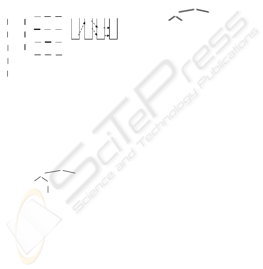
Example 1. Consider the document tree T shown in
Figure 3 and the query tree q shown in Figure 4.
Corresponding to the three leaf nodes in q, we have
three paths: P
1
: q
3
→ q
2
→ q
1
; P
2
: q
4
→ q
2
→ q
1
; and
P
3
: q
5
→ q
1
. When we apply TwigStack to T and q,
the stacks associated with the nodes in q will be
changed as follows.
Step 1 - 3: By the first iteration of the main while-
loop, q
1
is selected and then v
1
is pushed onto
S(q
1
). By the second iteration, q
2
will be
chosen since after the first iteration L(q
1
)
becomes empty and so we cannot find a v in
L(q
1
), which is an ancestor of next(L(q
2
)) =
v
2
. (See line 12 in getNext.) Therefore, v
2
goes into S(q
2
). For the same reason, q
3
will
be chosen by the third iteration and
next(L(q
3
)) = v
3
goes into S(q
3
). Since q
3
is a
leaf node, we get the first matching path (for
P
1
): v
3
→ v
2
→ v
1
. See Figure 5(a) for
illustration.
Step 4: By the fourth iteration, q
4
is selected and
next(L(q
4
)) = v
3
is pushed onto S(q
4
)) as
shown in Figure 5(b). We get the second
matching path (for P
2
): v
3
→ v
2
→ v
1
.
Step 5: By the fifth iteration, q
2
is chosen again.
Then, next(L(q
2
)) = v
4
is put on the top of
S(q
2
) as shown in Figure 5(c). Remember
that after each iteration, the pointer for the
WEBIST 2007 - International Conference on Web Information Systems and Technologies
8
corresponding L(q
act
) is shifted to the next
element.
Step 6: By the sixth iteration, q
3
is selected once
again and next(L(q
3
)) = v
5
will be put onto
S(q
3
). But before that, v
3
is popped out since
RightPos(v
3
) < LeftPos(v
3
) (see line 7 in
TwigStack.) The stacks are changed as shown
in Figure 5(d), which shows another two
paths matching P
1
: v
5
→ v
4
→ v
1
and v
5
→ v
2
→ v
1
. They are represented in the compact
form.
Step 7: By the seventh iteration, q
4
is selected for the
second time and next(L(q
4
)) = v
5
is pushed
onto S(q
4
). Before this operation, v
3
is first
popped out. The new stacks are shown in
Figure 5(e), from which we will get two new
matching paths (for P
2
): v
5
→ v
4
→ v
1
and v
5
→ v
2
→ v
1
.
Step 8: By the eighth iteration, q
5
is chosen and
next(L(q
5
)) = v
2
is put on the top of S(q
5
) as
shown in Figure 9(f). It shows the first
matching path for P
3
: v
2
→ v
1
.
Step 9: By the ninth iteration, q
5
is chosen once
again and next(L(q
5
)) = v
4
is put on the top of
S(q
5
) as shown in Figure 5(g). It shows the
second matching path for P
3
: v
4
→ v
1
.
Step 10:By the ninth iteration, q
5
is chosen for the
third time and next(L(q
5
)) = v
6
is put on the
top of S(q
5
) as shown in Figure 5(h). It shows
the second matching path for P
3
: v
6
→ v
1
. We
notice that in this step, q
2
will not be selected
although L(q
5
) = {v
6
} is not empty. It is
because both L(q
3
) and L(q
4
) are empty and
the condition (i) in the previous section
cannot be satisfied.
The time complexity of the algorithm can be
analyzed as follows.
Let n
i
be the size of L(q
i
). Then, the main while-
loop in TwigStack will be iterated
∑
=
m
i
i
n
1
times since
the termination condition of this while-loop is when
all the elements in all L(q
leaf
)’s are exhausted. In
each iteration, the procedure getNext will be invoked
and all the nodes in the query tree will be accessed.
Let λ
ijk
be the number of elements in L(q
k
) checked
when node q
k
is visited during the (i, j)-th execution
of getNext. Then, the worst-case cost is bounded by
O(
()
∑∑ ∑
== =
+
m
i
n
j
m
k
ijk
i
11 1
1
λ
)
= O(
∑∑ ∑
== =
m
i
n
j
m
k
i
11 1
1 ) + O(
∑∑ ∑
== =
m
i
n
j
m
k
ijk
i
11 1
λ
)
= O(m
2
⋅n) + O(m⋅n) = O(m
2
⋅n).
Here we should remark that O(
∑∑ ∑
== =
m
i
n
j
m
k
ijk
i
11 1
λ
)
cannot be larger than m⋅n since at most m⋅n elements
may be pushed on to the stacks.
Applying the above method to another algorithm
TwigStackXB in (Bruno and et al, 2002), which is an
extension of TwigStack for general cases, we get the
same time complexity.
3 REMOVING REDUNDANCY
FORM TWIGSTACK
Now we begin to discuss how TwigStack can be
improved. As with TwigStack, we will associate
each node q
i
in q with a data stream L(q
i
), but with
the following conditions satisfied:
(i) For each v ∈ L(q
i
), v matches the predicate at q
i
.
(ii) Let
1
i
q , ...,
k
i
q be the children of q
i
. v has a
descendant v’ matching
j
i
q for j ∈ {1, ..., k}.
(iii)Each
j
i
q recursively satisfies (ii).
Obviously, these three conditions correspond to
the two properties (i) and (ii) given in the previous
section, for any node going onto a stack. Nothing is
new. However, not like getNext in TwigStack, which
chooses nodes from q to handle and each time finds
a next v in T to be put in some stack (by multiple
S(q
5
) S(q
4
) S(q
3
) S(q
2
) S(q
1
)
v
3
v
2
v
1
v
3
v
3
v
2
v
1
S(q
5
) S(q
4
) S(q
3
) S(q
2
) S(q
1
)
(a) (b)
(c)
(d)
(e) (f)
v
3
v
3
v
4
v
2
v
1
v
5
v
3
v
4
v
2
v
1
v
5
v
5
v
4
v
2
v
1
v
5
v
5
v
4
v
2
v
1
v
2
(g) (h)
Figure 5: Sample trace.
v
5
v
5
v
4
v
2
v
1
v
4
v
2
v
5
v
5
v
4
v
2
v
1
v
6
STACK ENCODING REVISITED
9

executions), we generate all L(q
i
)’s in one scan,
which enables us to avoid a great number of
repeated accesses to query nodes.
In the following, we will use T’ to represent a
subtree of T, which contains only those nodes
matching some node in q.
We will maintain two m × n (m = |q|, n = |T’|)
matrices, defined as below.
1. The nodes in both q and T’ are numbered in
postorder, and the nodes v are then referred to
by their postorder numbers, denoted as post(v).
2. In the first matrix, each entry c
ij
(i ∈ {1, ..., m},
j ∈ {1, ..., n}) has value 0 or 1. If c
ij
= 1, it
indicates that i ∈ L(j) and for each child of i, j
has a descendant satisfying the predicate at it.
Otherwise, c
ij
= 0. This matrix is denoted by
c(q, T’).
3. In the second matrix, each entry d
ij
(i ∈ {1, ...,
m}, j ∈ {1, ..., n}) is defined as follows. If j has
a descendant j’ such that c
ij’
= 1, then d
ij
= 1;
otherwise d
ij
= 0. This matrix is denoted by d(q,
T’). In addition, a node itself is considered to be
one of its ancestors.
These two matrices can be established by using
an algorithm called matrixGeneration(T’, q),
presented below.
Initially, c
ij
= 0 and d
ij
= 0 for all i and j. During
the execution of the algorithm, the values of c
ij
’s will
be changed according to (2) and (3) described
above; and d
ij
’s will be changed to record whether a
node j in T’ has a descendant j’ that matches a
certain node i in q.
Algorithm matrixGeneration(T’, q)
Input: tree T’ (with nodes 1, ..., n) and tree q (with
nodes 1, ..., m)
Output: c(q, T’) with values created.
begin
1. for u := 1, ..., m do {
2. for v := 1, ..., n do
3. {if v satisfies the predicate at u then
4. let u
1
, ..., u
k
be the children of u;
5. if
vu
d
1
∧ ...
vu
k
d ∧ = 1 then c
uv
← 1;
6. }
7. let v
1
, v
2
, ..., v
h
be the nodes such that
pu
v
c = 1 (1
≤ p
≤
h);
8. let {w
1
, ..., w
r
} be a set such that each node in it
is an ancestor of some v
p
(1 ≤ p ≤ h). Set
l
uw
d = 1
for each w
l
(1 ≤ l ≤ r).
9. }
end
To see how the above algorithm works, we
should first notice that both T’ and q are both
postorder-numbered. Therefore, the algorithm
proceeds in a bottom-up way (see line 1 and 2). For
any node u in q and any node v in T’, if v satisfies
the predicate at u, we will check each child u
i
of u to
see whether there exists a descendant of v that
matches u
i
(see line 5). If it is the case, c
uv
will be set
to 1.
In line 7 and 8, we change d
ij
’s according to the
newly changed c
ij
’s.
Example 2. As an example, consider the trees T and
q shown in Figure 3 and 4 once again. Since each
node in T matches a node in q, we have T’ = T. In
addition, the nodes of T and q are postorder
numbered as shown in Figure 6(a) and (b),
respectively.
When we apply the above algorithm to these two
trees, c(q, T) and d(q, T) will be created and changed
in the way as illustrated in Figure 7, in which each
step corresponds to an execution of the outmost for-
loop.
In step 1, we show the values in c(q, T) and d(q,
T) after node 1 in q is checked against every node in
T. Since node 1 in q matches node 1 and 2 in T, c
11
and c
12
are all set to 1. Meanwhile, for all those
nodes that are an ancestor of 1 or 2 in T, the
corresponding entries in d(q, T) will be changed. So
we have all d
11
, d
12
, d
13
, d
14
, and d
16
set to 1 (see line
7 and 8).
In step 2, the algorithm generates the matrix
entries for node 2 in q, which is done in the same
way as for node 1 in q.
In step 3, node 3 in q will be checked against
every node in T, but matches only node 4 in T. Since
it is an internal node, its children will be further
checked. For this purpose, we will check both d
14
and d
24
since node 3 in q has two child nodes
postorder-numbered with 1 and 2, respectively.
Since d
14
= d
24
= 1, we set c
34
to 1. Accordingly, d
34
and d
36
are also set to 1.
In step 4, we will set c
43
, c
44
and c
45
to 1 since
node 4 in q is just a leaf node and matches node 3, 4,
and 5 in T. So d
43
, d
44
, d
45
, and d
46
will be
accordingly set to 1.
In step 5, since node 5 in q matches node 6 in T,
and both d
36
and d
46
are equal to 1 (we remark that
A v
1
B v
2
v
6
B
C v
3
v
4
B
v
5
C
Figure 6: Postorder numbering.
1
2
3
4
5
6
4
5 A q
1
B q
2
q
5
B
C q
3
q
4
C
1
2
3
WEBIST 2007 - International Conference on Web Information Systems and Technologies
10

node 3 and 4 in q are the child nodes of node 5), we
set c
56
and then d
56
to 1.
In the following discussion, we use T instead of
T’ to simplify the notation. The reader should notice
that it refers to the subtree of T containing only those
nodes that match some node in q.
Proposition 1. Algorithm matrixGeneration(T, q)
computes the values in c(q, T) and d(q, T) correctly.
Proof. We prove the proposition by induction on the
sum of the heights of T and q, h. Without loss of
generality, assume that height(T) ≥ 1 and height(q)
≥ 1.
Basic step. When h = 2, the proposition trivially
holds.
Induction hypothesis. Assume that when h = l, the
proposition holds.
Consider T = <t; T
1
, ..., T
k
> and q = <p; P
1
, ...,
P
g
> with height(T) + height(q) = l + 1, where t (p) is
the root of T (q, resp.) and T
1
, ..., T
k
(P
1
, ..., P
g
) are
the subtrees of t (p, resp.). Obviously, we have
height(T
i
) + height(q) ≤ l and height(T) + height(P
j
)
≤ l. Therefore, in terms of the induction hypothesis,
the algorithm correctly computes the values in c(q,
T
i
) and d(q, T
i
), as well as the values in c(P
j
, T) and
d(P
j
, T) (i = 1, ..., k; j = 1, ..., g). Assume that 1, ...,
m are the postorder numbers of the nodes in q, and 1,
..., n are the postorder numbers of the nodes in T.
Then, the values for c
ij
(i = 1, ..., m - 1; j = 1, ..., n -
1) and d
ij
(i = 1, ..., m - 1; j = 0, ..., n - 2) are all
correctly generated. Now we will check c
in
and d
i(n-1)
(i = 1, ..., m), as well as c
mj
(j = 1, ..., n) and d
mj
(j =
0, ..., n - 1) to see whether they can be correctly
produced. Let i
1
, ..., i
s
be the children of i. If i
matches n, for each i
f
(1 ≤ f ≤ s),
ni
f
d ’s will be
checked. If we have
ni
d
1
∧ ... ∧
ni
s
d = 1, we set c
in
to
1; otherwise 0 (see line 5). According to the
induction hypothesis, all such
ni
f
d ’s are correctly
generated. Therefore, c
in
(i = 1, ..., m) is correctly
created, so is d
i(n-1)
(i = 1, ..., m). A similar analysis
applies to c
mj
(j = 1, ..., n) and d
mj
(j = 0, ..., n - 1).
Proposition 2. Algorithm matrixGeneration(T, q)
requires O(n⋅m) time and space, where n = |T| and m
= |q|.
Proof. During the whole process, against each node
u in q, all the nodes v in T is checked and for each v
all its children will be examined. Therefore, this part
of time is bounded by
O(
∑∑
==
m
u
n
v
v
d
11
) = O(
∑
=
m
u
n
1
) = O(n⋅m),
where d
v
represents the outdegree of node v in T.
In addition, after each u in q is checked, for all
those nodes in T, which are an ancestor of some
node that matches u, the corresponding matrix
entries in d(q, T) will be established. But this
operation needs only O(n) time if we proceeds as
follows. Each time we search T bottom-up from a
node v that matches u to find all its ancestors, we
mark each node encountered and stop whenever we
meet such a mark (made by a previous searching).
So at most O(n) nodes will be checked and the total
time of this part of operations is bounded by O(n⋅m).
Obviously, to maintain c(q, T) and d(q, T), we
need O(n⋅m) space.
In terms of the matrix c(q, T), it is an easy task to
create L(q
i
) for each q
i
in q as illustrated in Figure
8(a).
Figure 8(b) is the same as Figure 8(a). But in this
figure we use node names in L(q
i
) instead of their
step 1:
1 2 3 4 5 6
1
2
3
4
5
1 1 0 0 0 0
0 0 0 0 0 0
0 0 0 0 0 0
0 0 0 0 0 0
0 0 0 0 0 0
c(q, T):
1 2 3 4 5 6
1
2
3
4
5
1 1 1 1 0 1
0 0 0 0 0 0
0 0 0 0 0 0
0 0 0 0 0 0
0 0 0 0 0 0
d(q, T):
step 2:
1 2 3 4 5 6
1
2
3
4
5
1 1 0 0 0 0
1 1 0 0 0 0
0 0 0 0 0 0
0 0 0 0 0 0
0 0 0 0 0 0
c(q, T):
1 2 3 4 5 6
1
2
3
4
5
1 1 1 1 0 1
1 1 1 1 0 1
0 0 0 0 0 0
0 0 0 0 0 0
0 0 0 0 0 0
d(q, T):
step 3:
1 2 3 4 5 6
1
2
3
4
5
1 1 0 0 0 0
1 1 0 0 0 0
0 0 1 1 0 0
0 0 0 0 0 0
0 0 0 0 0 0
c(q, T):
1 2 3 4 5 6
1
2
3
4
5
1 1 1 1 0 1
1 1 1 1 0 1
0 0 1 1 0 1
0 0 0 0 0 0
0 0 0 0 0 0
d(q, T):
step 4:
1 2 3 4 5 6
1
2
3
4
5
1 1 0 0 0 0
1 1 0 0 0 0
0 0 1 1 0 0
0 0 1 1 1 0
0 0 0 0 0 0
c(q, T):
1 2 3 4 5 6
1
2
3
4
5
1 1 1 1 0 1
1 1 1 1 0 1
0 0 1 1 0 1
0 0 1 1 1 1
0 0 0 0 0 0
d(q, T):
step 5:
1 2 3 4 5 6
1
2
3
4
5
1 1 0 0 0 0
1 1 0 0 0 0
0 0 1 1 0 0
0 0 1 1 1 0
0 0 0 0 0 1
c(q, T):
1 2 3 4 5 6
1
2
3
4
5
1 1 1 1 0 1
1 1 1 1 0 1
0 0 1 1 0 0
0 0 1 1 1 1
0 0 0 0 0 1
d(q, T):
Figure 7: Sample trace.
STACK ENCODING REVISITED
11

postorder numbers. We will use the node names in
the subsequent discussion to avoid any confusion.
Concerning L(q
i
), we should pay attention to the
following:
(1) The nodes (represented by their quadruple) in
L(q
i
) are sorted by their (DocId, LeftPos) values
(not according to their postorder numbers).
(2) Each node in L(q
i
) satisfies the condition (i) and
(ii) given in 2.2.
Using such a data structure, the algorithm
TwigStack can be substantially improved. The main
idea is a depth-first searching of q. To this end, we
use a stack to control the process. Each entry in the
stack is a pair (q
i
, v
j
), where q
i
∈ q and v
j
∈ T.
Finally, we notice that getNext( ) will not be used
since all the values to be produced by executing
getNext( ) are pre-calculated and incorporated into
L(q
i
)’s. In addition, each node q
i
in q is associated
with its preorder number, denoted as pre(q
i
), which
will be used in the following algorithm. In Figure 9,
we show the preorder numbering of q.
Algorithm
RefinedTwigStack(q)
(*phase 1*)
1.Repeat the following until all
L(q
i
) become empty;
2. { let
pre(q
i
) be the least such that L(q
i
) is not empty;
3. push(
stack, (q
i
, next(L(q
i
)));
4. while ¬ empty(
stack) do
{(
u, v) ← pop(stack);
6. if (
u
is not the root) then
7.
cleanStack(S(parent(u)), LeftPos(v));
8. if (
u
is the root of q) ∨ ¬ empty(S(parent(u)))
9. then
10
. {cleanStack(S(u), LeftPos(v));
11. push(
S(u), v, pointer to top(S(parent(u)));
advance(L(u));
12. if (
u is a leaf node) then
13. { output all the matching paths (stored in stacks)
in the compact form; pop(
S(u));}
14. }
15. else advance(L(u));
16. let
q
1
, ..., q
l
be the children of u;
17. for
j = l to 1 do
18. {while
next(L(q
j
) is not a descendant of v do
adavance(L(q
j
);
19. push(stack, (
q
j
, next(L(q
j
)));}
20.}}
(*phase 2*)
21.
mergeAllPathSolutions();
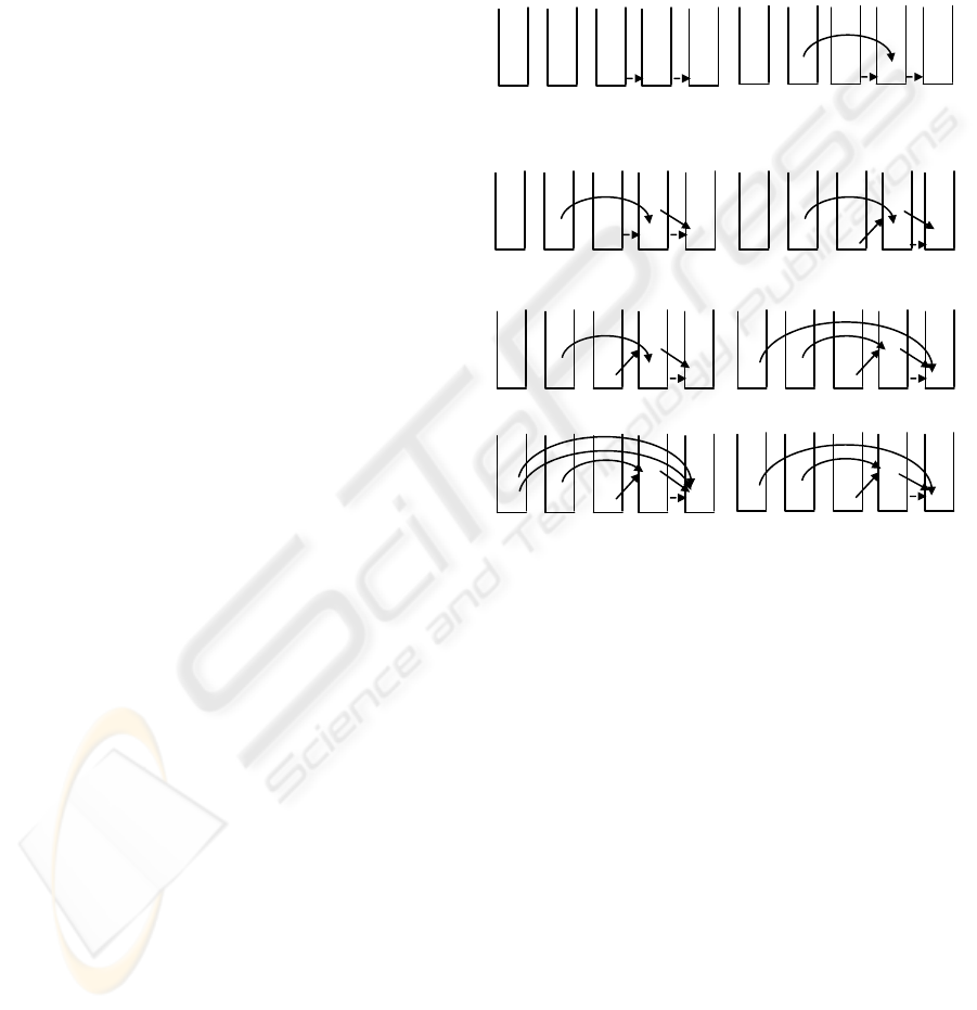
Example 3. Continue with Example 2.
By using our method, we will first generate
L(q
i
) for
each
q
i
as shown in Figure 8(b). Then, we will search the
twig pattern
q as follows.
Step 0: At the very beginning, the node
q
1
has the least
LeftPos value and
L(q
1
) is not empty. Push (q
1
,
v
1
) into stack.
Step 1 - 3: In the following while-loop, the whole query
tree will be traversed in depth-first fashion.
When we meet
q
3
, the stacks will be changed as
shown in Figure 10(a). Since
q
3
is a leaf node, we
get the first matching path (for
P
1
): v
3
→ v
2
→ v
1
.
Step 4: When we meet
q
4
, another leaf node, the stacks
will be changed as shown in Figure 10(b). We get
the second matching path (for
P
2
): v
3
→ v
2
→ v
1
.
Step 5:
q
5
is visited. The stacks are changed as shown in
Figure 10(c). Since
q
4
is a leaf node, we get the
third matching path (for
P
3
): v
2
→ v
1
.
Step 6: Now
stack (used to control the searching of q) is
empty. We will try to find another node (in
q)
with the least LeftPos value and a non-empty list.
It is q
2
. In L(q
2
), we have one element left: {v
4
}.
Push (
q
2
, v
4
) into stack.
q
2
is visited once again. The stacks will be
changed as shown in Figure 10(d).
Step 7:
q
3
is visited once again. The stacks will be
changed as shown in Figure 10(e). (We notice that
before
v
5
is pushed onto S(q
3
), v
3
is popped out.)
From this, we get another two paths matching
P
1
:
v
5
→ v
4
→ v
1
and v
5
→ v
2
→ v
1
. They are
represented in the compact form.
Step 8: q
4
is visited once again. The stacks will be
changed as shown in Figure 10(f). (We notice that
before
v
5
is pushed onto S(q
4
), v
3
is popped out.)
From this, we get another two paths matching P
2
:
v
5
→ v
4
→ v
1
and v
5
→ v
2
→ v
1
. They are
represented in the compact form.
Step 9:
Stack becomes empty once again. This time q
5
is
chosen and in
L(q
5
) we still have two elements:
{
v
4
, v
6
}. Push (q
5
, v
4
) into stack.
3
{3, 4}
{6}
{1, 2}
4
5 A q
1
B q
2
q
5
B
C q
3
q
4
C
1
2
{1, 2}
{3, 4, 5}
{v
2
, v
4
, v
6
}
{v
2
, v
4
}
{v
3
, v
5
} {v
3
, v
5
}
{v
1
}
A q
1
B q
2
q
5
B
C q
3
q
4
C
Figure 8: Illustration for L(q
i
)’s.
5
1
A q
1
B q
2
q
5
B
C q
3
q
4
C
3
4
2
Figure 9: Preorder numbering.
WEBIST 2007 - International Conference on Web Information Systems and Technologies
12
q
5
is visited for the second time. The new status
of the stacks is shown in Figure 10(g). From this,
we get the second path matching
P
3
: v
4
→ v
1
.
Step 10: Stack becomes empty for the third time, and q
5
is
chosen once again since we still have an element
in
L(q
5
): {v
6
}. Push (q
5
, v
6
) into stack.
q
5
is visited for the second time. The new status
of the stacks is shown in Figure 10(h) (before
v
6
is pushed onto
S(q
5
), v
2
and v
4
are popped out.)
From this, we get the third path matching P
3
: v
6
→ v
1
. □
From the above example, we can see that our
algorithm generates the same paths as TwigStack
although the order of such paths’s generation is
different. More importantly, in our algorithm
getNext is not used, which is replaced with
matrixGeneration that is performed only once.
In the following, we prove the algorithm’s
correctness and analyze its time complexity.
Proposition 3. Let T and q be the document and
query tree, respectively. RefindTwigStack generates
all the matching paths (in T) for every root-to-leaf
path in q.
Proof. In order to prove the proposition, we need to
explain
(i) Every path (in T) found by RefinedTwigStack
must match a root-to-leaf path in q.
(ii) Any path (in T), if it matches a root-to-leaf path
in q and each of its nodes satisfies the condition
(i) and (ii) given in 2.2, must be found by
RefinedTwigStack.
Proof of (i). To see that (i) holds, we notice the
following two properties of the algorithm:
(1) Any node v in any L(q
i
) satisfies the condition (i)
and (ii) given in 2.2.
(2) Any node v put in a S(q
i
) satisfies the condition
below:
Let q’ be the parent of q
i
. The node on the top of
S(q’) must be an ancestor of v.
So each time when we meet a leaf node q’’, all
the paths found must match the path from the root of
q to q’’.
Proof of (ii). Let P = q
1
→
q
2
... →
q
m
be a path in
q. Let {t
1
, t
2
, ..., t
m
} be a set of nodes lying on a path
in T, which makes up a matching path of P with
each t
i
satisfying the condition (i) and (ii) given in
2.2. But this matching path has not been found by
RefinedTwigStack. Then, there exists a k such that
all t
j
(k
≤
j
≤
m) do not have a chance to be put onto
the corresponding stacks. First, we notice that k > 1
since t
1
must appear in L(q
1
) and will be definitely
put onto S(q
1
) during the computation process. Now
we consider t
k
with k > 1, which does not have a
chance to be put onto S(q
k
). In terms of line 8 in
RefinedTwigStack, we must have S(q
k+1
) = {} when
we try to put t
k
onto S(q
k+1
). This implies that t
k-1
must have been popped out at a earlier time point
when we try to put another node t’ onto S(q
k
) with
RightPos(t
k-1
) < LeftPos(t’). But we have obviously
LeftPos(t’) < LeftPos(t
k
). So we have RightPos(t
k-1
)
< LeftPos(t
k
), which contradicts fact that t
k-1
is an
ancestor of t
k
. From this analysis, we know that t
k
has a chance to be put onto S(q
k
). The same analysis
applies to t
k+1
, ..., t
m
. This completes the proof.
The time complexity of RefinedTwigStack is
easy to analyze. In the whole process, each node v in
a L(q
i
) is accessed only once. So the total cost is
bounded by
O(
()
∑
=
m
i
i
qL
1
) = O(m⋅n)
4 GENERAL CASES
The method discussed in Section 3 can be easily
extended to handle general cases that a query tree
contains both c-edges and d-edges. For this purpose,
we define a third matrix p(q, T) as follows.
An entry p
ij
= 1 indicates that there exists some
child k of j, which ‘matches’ i, i.e., c
ik
= 1;
otherwise, p
ij
= 0.
S(q
5
) S(q
4
) S(q
3
) S(q
2
) S(q
1
)
v
3
<
v
2
v
1
v
3
v
3
v
2
v
1
S(q
5
) S(q
4
) S(q
3
) S(q
2
) S(q
1
)
(a) (b)
(c) (d)
(e) (f)
v
3
v
3
v
2
v
1
v
2
v
3
v
3
v
4
v
2
v
1
v
2
v
5
v
3
v
4
v
2
v
1
v
2
v
5
v
5
v
4
v
2
v
1
v
2
(g) (h)
Figure 10: Sample trace.
v
5
v
5
v
4
v
2
v
1
v
4
v
2
v
5
v
5
v
4
v
2
v
1
<
v
6
STACK ENCODING REVISITED
13

Accordingly, the algorithm matrixGeneration
should be slightly changed so that the manipulation
of p(q, T) is involved.
Algorithm generalMatrixGeneration(T, q)
Input: tree
T (with nodes 1, ..., n) and tree q (with nodes 1,
...,
m)
Output:
c(q, T) with values created.
begin
1. for u := 1, ..., m do {
2. for
v := 1, ..., n do
3. {if
v satisfies the predicate at u then
4. let
u
1
, ..., u
k
be the c-children of u;
5. let
u
1
’, ..., u
g
’ be the d-children of u;
6. if
vu
p
1
∧ ... ∧
vu
k
p = 1 and
vu
d
'
1
∧ ... ∧
vu
k
d
'
= 1
7. then c
uv
← 1;}
8. let v
1
, v
2
, ..., v
h
be the nodes such that
p
uv
c = 1 (1 ≤ p
≤ h);
9. let {
w
1
, ..., w
r
} be a set such that each node in it is an
ancestor of some
v
p
(1 ≤ p ≤ h). Set
l
uw
d
= 1 for each w
l
(1 ≤
l ≤ r).
10. let {
t
1
, ..., t
s
} be a set such that each node in it is a
parent of some
v
p
(1 ≤ p ≤ h). Set
l
ut
d = 1 for each t
l
(1
≤ l ≤ s).
11. }
end
Since each node u in q may have both c- and d-
children, each time when checking it against a node
v in T we need to check the corresponding entries in
both d(q, T) and p(q, T) (see line 6). In addition,
besides the computation of new values for some
entries in d(q, T) in each step, we need also to
compute new values for the corresponding entries in
p(q, T) (see line 10).
5 CONCLUSION
In this paper, a new method is discussed, which
substantially improves the method proposed in
(Bruno and et al, 2002) for doing twig joins that are
identified as a core operation for query evaluation in
XML databases. Concretely, our method improves
the algorithm TwigStack and TwigStackXB presented
in (Bruno and et al, 2002) from O(m
2
⋅n) to O(m⋅n),
where m and n are the sizes of the query tree and
document tree, respectively. In addition, a system
implementation and experiments are reported, which
shows that our method uniformly outperforms
TwigStack, completely conforming to the conducted
theoretic analysis.
ACKNOWLEDGEMENTS
The author is supported by NSERC 239074-01
(242523) (Natural Sciences and Engineering Council
of Canada).
REFERENCES
S. Al-Khalifa, H.V. Jagadish, N. Koudas, J.M. Patel, D.
Srivastava, and Y. Wu (2002). Structureal Joins:
Aprimitive for efficient XML query pattern matching,
in
Proc. of IEEE Int. Conf. on Data Engineering.
N. Bruno, N. Koudas, and D. Srivastava (2002). Holistic
Twig Hoins: Optimal XML Pattern Matching, in
Proc.
SIGMOD Int. Conf. on Management of Data
,
Madison, Wisconsin, June 2002, pp. 310-321.
D. D. Chamberlin, J.Clark, D. Florescu and M. Stefanescu
(1999). XQuery1.0: An XML Query Language,
http://www.w3.org/ TR/query-datamodel/.
D. D. Chamberlin, J. Robie and D. Florescu (2000). Quilt:
An XML Query Language for Heterogeneous Data
Sources,
WebDB 2000.
A. Deutch, M. Fernandex, D. Florescu, A. Levy, D.Suciu
(1999). A Query Language for XML, WWW'99.
D. Florescu and D. Kossman, Storing and Querying
(1999). XML data using an RDMBS, IEEE Data
Engineering Bulletin
, 22(3):27-34.
J. McHugh, J. Widom (1999) Query optimization for
XML, in Proc. of VLDB.
J. Shanmugasundaram, K. Tufte, C. Zhang, G. He, D.J.
Dewitt, and J.F. Naughton (1999). Relational
databases for querying XML documents: Limitations
and opportunities, in Proc. of VLDB.
The Tukwila System (1999), available from U. of
Washington http:/ /data.cs.washington.edu/integration
/tukwila/.
The Niagara System (2000), available from U. of
Wisconsin http:// www.cs.wisc.edu/niagara/.
H. Wang, S. Park, W. Fan, and P.S. Yu (2003). ViST: A
Dynamic Index Method for Querying XML Data by
Tree Structures,
SIGMOD Int. Conf. on Management
of Data
, San Diego, CA., June 2003.
H. Wang and X. Meng (2005) On the Sequencing of Tree
Structures for XML Indexing, in
Proc. Conf. Data
Engineering
, Tokyo, Japan, April, 2005, pp. 372-385.
World Wide Web Consortium (1999). XML Path
Language (XPath), W3C Recommendation, Version
1.0, November 1999. See
http://www.w3.org/TR/xpath.
World Wide Web Consortium (2001) XQuery 1.0: An
XML Query Language, W3C Recommendation,
Version 1.0, Dec. 2001. See http://www.w3.org/TR/
xquery.
C. Zhang, J. Naughton, D. Dewitt (2001) Q. Luo, and G.
Lohman, on Supporting containment queries in
relational database management systems, in
Proc. of
ACM SIGMOD
, 2001.
WEBIST 2007 - International Conference on Web Information Systems and Technologies
14
