A HYPER-HEURISTIC FOR SCHEDULING INDEPENDENT JOBS

IN COMPUTATIONAL GRIDS

Juan Antonio Gonzalez, Maria Serna and Fatos Xhafa

Departament de Llenguatges i Sistemes Informtics

Universitat Politcnica de Catalunya

Campus Nord, Ed. Omega, C/Jordi Girona 1-3

08034, Barcelona, Spain

Keywords:

Scheduling, Grid Computing, Heuristic methods, Immediate mode, Batch mode.

Abstract:

In this paper we present the design and implementation of an hyper-heuristic for efﬁciently scheduling in-

dependent jobs in Computational Grids. An efﬁcient scheduling of jobs to Grid resources depends on many

parameters, among others, the characteristics of the Grid infrastructure and job characteristics (such as com-

puting capacity, consistency of computing, etc.). Existing ad hoc scheduling methods (batch and immediate

mode) have shown their efﬁcacy for certain types of Grids and job characteristics. However, as stand alone

methods, they are not able to produce the best planning of jobs to resources for different types of Grid resources

and job characteristics.

In this work we have designed and implemented a hyper-heuristic that uses a set of ad hoc (immediate and

batch mode) scheduling methods to provide the scheduling of jobs to Grid nodes according to the Grid and job

characteristics. The hyper-heuristic is a high level algorithm, which examines the state and characteristics of

the Grid system (jobs and resources), and selects and applies the ad hoc method that yields the best planning

of jobs to Grid resources. The resulting hyper-heuristic based scheduler can be thus used to develop network-

aware applications that need efﬁcient planning of jobs to resources.

The Hyper-heuristic has been tested and evaluated in a dynamic setting through a prototype of a Grid simulator.

The experimental evaluation showed the usefulness of the hyper-heuristic in planning of jobs to resources as

opposed to planning without knowledge of the Grid and jobs characteristics.

1 INTRODUCTION

The Computational Grid (CG) has emerged as a new

paradigm for large scale distributed applications (Fos-

ter and Kesselman, 1998; Foster et al., 2001). A

CG logically uniﬁes in a single computational unit

geographically distributed and highly heterogeneous

resources, which are interconnected through hetero-

geneous networks. The CG can thus be viewed as

a “type of parallel and distributed system that en-

ables the sharing, selection, and aggregation of geo-

graphically distributed autonomous resources dynam-

ically depending on their availability, capability, per-

formance, cost, and users’ QoS requirements” (Foster

and Kesselman, 1998). As a matter of fact, the par-

allel and distributed nature of CGs was the ﬁrst ex-

ploited feature for solving combinatorial optimization

problems that are computationally hard (Casanova

and Dongarra, 1998; Wright, 2001; Linderoth and

Wright, 2003). More generally, during the last years,

Grid computing has motivated the development of

large scale applications that need the large computing

capacity offered by the Grid. Many Grid-enabled ap-

plication as well as many Grid-based infrastructures

are being reported in the Grid computing domain.

In order to achieve the Grid as a single computa-

tional unit many complex issues are nowadays being

investigated. One key issue is to efﬁciently beneﬁt

from the parallel nature of Grid systems. The large

computing capacity offered by Grids not necessar-

ily yields to high performance applications. Indeed,

efﬁcient techniques that allocate jobs/applications to

Grid resources are necessary. The resource allocation

problem is known to be computationally hard (Garey

and Johnson, 1979). Although the scheduling prob-

lems are among most studied problems in combinato-

128

Antonio Gonzalez J., Serna M. and Xhafa F. (2007).

A HYPER-HEURISTIC FOR SCHEDULING INDEPENDENT JOBS IN COMPUTATIONAL GRIDS.

In Proceedings of the Second International Conference on Software and Data Technologies - PL/DPS/KE/WsMUSE, pages 128-135

DOI: 10.5220/0001328701280135

 SciTePress

rial optimization, the heterogenous and dynamic char-

acteristics of Grids makes the problem very complex

for Grid environments. For instance, a Grid can con-

nect PCs, LANs and Supercomputers and jobs of very

different workload can arrive in the Grid. Moreover,

job scheduling in Grids is a large scale optimization

problem due to the large number of jobs that could ar-

rive in the Grid and of the large number of Grid nodes

that could potentially participate in the planning of

jobs. Therefore, although useful, the techniques used

in traditional scheduling may fail to produce efﬁcient

planning in Grids since they are not grid-aware, that

is, do not have knowledge of the characteristics of the

underlaying Grid infrastructure.

Given the dynamic nature of the grid systems,

any scheduler should provide allocations of jobs to

resources as fast as possible. Therefore, schedulers

based on very efﬁcient methods are very important

especially in presence of time restrictions on job ex-

ecutions on the grid. Immediate and batch methods

fall into this type of methods since they distinguish

for their efﬁciency in contrast to more sophisticated

schedulers that could need larger execution times.

In the immediate mode, a job is scheduled as soon

as the job enters in the scheduler while in batch mode

jobs are grouped in a batch of jobs, which is sched-

uled according to a time interval speciﬁed by a map-

ping event. Thus, in immediate mode we are inter-

ested to schedule jobs without waiting for the next

time interval the scheduler will get activated or when

the job arrival rate is small having thus available re-

sources to execute jobs immediately. On the con-

trary, when the job arrival rate is high, resources are

most likely occupied with executing previously allo-

cated jobs, thus the batch mode could be activated. In

the immediate mode we consider the following ﬁve

methods: Opportunistic Load Balancing (OLB), Min-

imum Completion Time (MCT), Minimum Execution

Time (MET), Switching Algorithm (SA) and k-Percent

Best (kPB). The batch mode methods we consider are:

Min-Min, Max-Min, Sufferage and Relative Cost.

Ad hoc methods for for heterogenous computing

environments have been explored in several works

in the literature (Maheswaran et al., 1999; Abraham

et al., 2000; Braun et al., 2001; Wu and Shu, 2001).

Depending on the characteristics of the Grid resources

and jobs, these methods could present very different

performance. For instance, the MCT method per-

forms well for consistent computing environments,

however, it performs poorly for inconsistent com-

puting environments. Moreover, an ad hoc method

could perform well if the optimization criterion is the

makespan but could perform poorly if the optimiza-

tion criterion were the ﬂowtime. Thus, as stand alone

methods, these ad hoc methods are not able to pro-

duce the best planning of jobs to resources for differ-

ent types of Grid resources and job characteristics.

In this work we have designed and implemented

an hyper-heuristic that uses the above mentioned ad

hoc methods to achieve the best scheduling of jobs to

Grid nodes according to the Grid and job character-

istics. The hyper-heuristic is a high level algorithm,

which examines the state and characteristics of the

Grid system (jobs and resources), and applies the ad

hoc method that yields the best planning of jobs to

Grid resources.

Our starting point was the empirical evaluation of

the nine ad hoc methods using the static benchmark of

static instances (Braun et al., 2001). This benchmark

is intended for heterogenous environments and con-

sists of families of instances sharing common charac-

teristics regarding the consistency of computing, the

heterogeneity of jobs and heterogeneity of resources.

We run each of the nine ad hoc methods on 100 dif-

ferent instances of the benchmark to study the behav-

ior of these ad hoc methods and then we embed this

knowledge on the hyper-heuristic. The performance

of the hyper-heuristic is evaluated in a dynamic en-

vironment through a prototype of a Grid simulator.

The experimental study showed the usefulness of us-

ing the hyper-heuristic, which uses knowledge of the

underlying Grid (such as the degree of consistency

of computing, heterogeneity of jobs and heterogene-

ity of resources) in its decision-taking as opposed to

using ad hoc heuristics as stand alone methods or a

pure random choice method. The performance of the

hyper-heuristic is done with regard to three parame-

ters of the Grid system: makespan, ﬂowtime and re-

source utilization.

The rest of the paper is organized as follows. We

give in Section 2 a description of the job scheduling

in computational grids considered in this work. The

ad hoc methods used in the hyper-heuristic as well

as their evaluation is given in Section 3. The design

of the hyper-heuristic is given in Section 4 and some

computational results and evaluation is given in Sec-

tion 5. We end in Section 6 with some conclusions

and future work.

2 INDEPENDENT JOB

SCHEDULING IN GRIDS

The job scheduling problem in grids has many char-

acteristics in common with the traditional scheduling

problems. The objective is to efﬁciently map jobs to

resources; however, in a global, heterogenous and dy-

namic environment, such as grid environment, we re

A HYPER-HEURISTIC FOR SCHEDULING INDEPENDENT JOBS IN COMPUTATIONAL GRIDS

129

interested to ﬁnd a practically good planning of jobs

very fast. Moreover, unlike traditional scheduling in

which the makespan is the most important parame-

ter, we are also interested to optimize ﬂowtime and

resource utilization.

In this work we deal with the scheduling indepen-

dent jobs to resources. We describe this version next

and then give a formal deﬁnition of an instance of

the problem. Jobs have the following characteristics:

are originated from different users/applications, have

to be completed in unique resource (non-preemptive),

are independents and could also have their require-

ments over resources. This last characteristic is im-

portant if we would like to classify jobs originated in

data intensive or computing intensive applications.

On the other hand, resources could dynamically

be added/dropped from the Grid, can process one job

at a time and have their computing characteristics.

2.1 Expected Time to Compute

Simulation Model

In order to formalize the instance deﬁnition of the

problem, we use the ETC (Expected Time To Com-

pute) matrix model, see e.g. (Braun et al., 2001). This

model is used for capturing most important charac-

teristics of job and resources in distributed hetero-

geneous environments. In a certain sense, a good

planning jobs to resources will have to take into ac-

count the characteristics of jobs and resources. More

precisely, the Expected Time to Compute matrix,

ETC, has size nb

jobs × nb machines and its com-

ponents are deﬁned as ETC[i][ j] = the expected exe-

cution time of job i in machine j. ETC matrices are

then classiﬁed into consistent, inconsistent and semi-

consistent according to the consistency of computing

of resources: (a) consistency means that if a machine

executes a job faster than machine m

, then m

ex-

ecutes all the jobs faster than m

. If this holds for all

machines participating in the planning, the ETC ma-

trix is considered consistent ; (b) inconsistency means

that a machine is faster for some jobs and slower for

some others; and, (c) semi-consistency is used to ex-

press the fact that an ETC matrix can have a consistent

sub-matrix. In this case the ETC matrix is considered

semi-consistent. Notice that the variability in charac-

teristics of jobs and resources yields to different ETC

conﬁgurations allowing thus to simulate different sce-

narios from real life distributed applications.

2.2 Problem Deﬁnition

Under the ETC simulation model, an instance of the

problem consists of:

– A number of independent (user/application) jobs

to be scheduled.

– A number of heterogeneous machines candidates

to participate in the planning.

– The workload of each job (expressed in millions

of instructions).

– The computing capacity of each machine (ex-

pressed in mips –millions of instructions per sec-

ond).

– Ready time ready[m] –when machine m will have

ﬁnished the previously assigned jobs. (Measures

the previous workload of a machine.)

– The Expected Time to Compute matrix, ETC.

Note that this version of the problem does not in-

clude local policies of resources, time for data trans-

mission and possible job dependencies. Yet, this ver-

sion arises in many grid-based applications, such as

in simulations, massive data processing, which can be

divided into independent parts, which are mapped to

different grid nodes.

Optimization criteria. Several parameters could

be measured for a given schedule. Among these, there

are (S denotes a possible schedule):

(a) makespan (ﬁnishing time of latest job) deﬁned as

min

max{F

: j ∈ Jobs}.

(b) flowtime (sum of ﬁnishing times of jobs), that is,

min

∑

j∈Jobs

erage resource utilization. This last parameter is

deﬁned using the completion time of a machine,

which indicates the time in which machine m will

ﬁnalize the processing of the previous assigned

jobs as well as of those already planned for the

machine. Formally, it is deﬁned as follows:

completion[m] = ready[m] +

∑

j∈S

−1

(m)

ETC[ j][m].

Having the values of the completion time for the

machines, we can deﬁne the makespan, which is in

fact the local makespan by considering only the ma-

chines involved in the current schedule:

makespan = max{completion[i] | i ∈ Machines

′

Then, we deﬁne:

ICSOFT 2007 - International Conference on Software and Data Technologies

130

avg utilization =

∑

{i∈Machines}

completion[i]

makespan· nb machines

It should be noted that these parameters are very

important for grid systems. Makespan measures the

productivity of the grid system, the ﬂowtime mea-

sures the QoS of the grid system and resource utiliza-

tion indicates the quality of a schedule with respect to

the utilization of resources involved in the schedule

aiming to reduce idle time of resources.

3 AD HOC METHODS USED IN

THE HYPER-HEURISTIC

Several speciﬁc scheduling methods were considered

in the implementation of the hyper-heuristic. These

speciﬁc methods belongs to two families: immedi-

ate and batch mode. In the former we have methods

that schedule jobs to Grid resources as soon as they

enter in the Grid system, while in the later batches

of jobs are scheduled. Notice that disposing of these

two types of processing (immediate and batch) allows

us to better match the computational needs and re-

quirements of scheduling; thus, based on job charac-

teristics we could classify jobs as immediate-like or

batch-like.

3.1 Immediate Mode Methods

In the immediate mode we considered the following

ﬁve methods to be used in the hyper-heuristic: Oppor-

tunistic Load Balancing (OLB), Minimum Comple-

tion Time (MCT), Minimum Execution Time (MET),

Switching Algorithm (SA) and k-Percent Best (kPB).

OLB: This method assigns a job to the earliest idle

machine without taking into account the execution

time of the job in the machine. If two or more ma-

chines are available at the same time, one of them

is arbitrarily chosen. Usually this method is used in

scavenging grids. One advantage of this method is

that it tries to keep the machines as loaded as possi-

ble; however, the method is not aware of the execu-

tion times of jobs into machines, which is, certainly,

a disadvantage as regards the makespan and ﬂowtime

parameters.

MCT: This method assigns a job to the machine

yielding the earliest completion time (the ready times

of the machines are used). Note that a job could be

assigned to a machine that does not have the small-

est execution time for that job. This method is also

known as Fast Greedy, originally proposed for Smart-

Net system.

MET: This method assigns a job to the machine

having the smallest execution time for that job. Note

that unlike MCT, this method does not take into ac-

count the ready times of machines. Clearly, in grid

systems of different computing capacity resources,

this method could produce an unbalance by assign-

ing jobs to fastest resources. However, the advantage

is that jobs are allocated to resources that best ﬁt them

as regards the execution time.

SA: This method tries to overcome some limitations

of MET and MCT methods by combining their best

features. More precisely, MET is not good for load

balancing while MCT does not take into account exe-

cution times of jobs into machines. Essentially, the

idea is to use MET till a threshold is reached and

then use MCT to achieve a good load balancing. SA

method combines MET and MCT cyclically based on

the workload of resources.

In order to implement the method, let r

max

be the

maximum ready time and r

min

the minimum ready

time; the load balancing factor is then r

min

max

which takes values in [0,1]. Note that for r = 1.0

we have a perfect load balancing and if r = 0.0 then

there exists at least one idle machine. Further, we

use to threshold values r

(low) and r

(high) for r,

0 ≤ r

< r

≤ 1. Initially, r = 0.0 so that SA starts allo-

cating jobs according to MCT until r becomes greater

than r

; after that, MET is activated so that r becomes

smaller than r

and a new cycle starts again until all

jobs are allocated.

kPB: For a given job, this method considers a sub-

set of candidate resources from which the resource to

allocate the job is chosen. The candidate set consists

of m· k/100 best resources (with respect to execution

times) for the given job, for k, m/100 ≤ k ≤ 100. The

machine to allocate the job is taken the one from the

candidate set yielding the earliest completion time.

Note that for k = 100, kPB behaves as MCT and for

k = 100/m it behaves as MET. It should be noted that

this method could perform poorly if the subset of re-

sources is not within k% best resources for any of jobs

implying thus a large idle time.

3.2 Batch Mode Methods

We considered the following batch methods: Min-

Min, Max-Min, Sufferage and Relative Cost.

A HYPER-HEURISTIC FOR SCHEDULING INDEPENDENT JOBS IN COMPUTATIONAL GRIDS

131

Min-Min: This method starts by computing a ma-

trix of values completion[i][ j] for any job i and

machine j based on ETC[i][ j] and ready

values

(completion[i][ j] = ETC[i][ j]+ready[ j]). For any job

i, the machine m

yielding the earliest completion time

is computed by traversing the ith row of the comple-

tion matrix. Then, job i

with the earliest comple-

tion time is chosen and mapped to the corresponding

machine m

(previously computed). Next, job i

removed from Jobs and completion[i][ j] values ∀i in

Jobs and machine m

are updated. The process is re-

peated until there are jobs to be assigned.

Max-Min: This method is similar to Min-Min. The

difference is that once it is computed, for any job i,

the machine m

yielding the earliest completion time,

the i

with the latest completion time is chosen and

mapped to the corresponding machine. Note that this

method is appropriate when most of the jobs entering

the grid system are short. Thus, Max-Min would try

to schedule at the same time all the short jobs and

longest ones while Min-Min would schedule ﬁrst the

shortest jobs and then the longest ones implying thus

a larger makespan.

Sufferage: The idea behind this method is that bet-

ter scheduling could be obtained if we assign to a ma-

chine a job, which would “suffer” more if it were

assigned to any other machine. To implement this

method, the sufferage parameter of a job is deﬁned

as the difference between the second earliest comple-

tion time of the job in machine m

and the ﬁrst ear-

liest completion time of the job in machine m

. The

method starts by labelling all machines as available.

Then, in each iteration (of a while loop) a pending job

j is chosen to be scheduled. To this end, for job j,

the machines m

and m

and the sufferage value are

computed. If machine m

is available, then job j is as-

signed to m

. In case, m

is already executing another

job j

′

, then jobs j and j

′

will compete for machine m

;

the winner is the job of largest sufferage value. The

job loosing the competition will be considered once

all pending jobs have been analyzed.

Relative Cost: In allocating jobs to machines, this

method takes into account both the load balancing

of machines and the execution times of jobs in ma-

chines, that is, for a given job, ﬁnd the machine that

best matches job’s execution time. This last criterion

is known as matching proximity and is used, apart

from makespan, ﬂowtime and resource utilization for

measuring the performance of the allocation method.

Note that load balancing and matching proximity are

contradicting criteria. In order to ﬁnd a good trade-

off between them the method uses two parameters,

namely, static relative cost and dynamic relative cost.

Given a job i and machine j, the static relative cost γ

is deﬁned as γ

= ETC[i][ j]/etc

avg

, where:

etc avg

∑

j∈Machines

ETC[i][ j]/nb

machines.

This static parameter is computed once at the begin-

ning of the execution of the method. The dynamic

relative cost is computed at the beginning of each it-

eration k, as

= completion

(k)

[i][ j]/completion

avg

(k)

where:

completion avg

(k)

∑

j∈Machines

completion

(k)

[i][ j]

nb machines

At each iteration k, the best job i

best

is the one that

minimizes the expression (γ

i,m

∗

)

· γ

i,m

∗

, ∀i ∈ Jobs,

where

∗

= argmin{completion

(k)

[i][m] | m ∈ Machines}.

The value of α is ﬁxed to 0.5.

3.3 Evaluation of the Ad Hoc Methods

on a Static Benchmark

We empirically evaluated the performance of the nine

ad hoc methods presented above, using a benchmark

of static instances (Braun et al., 2001). The objec-

tive is to use the evaluation results for taking better

decisions in running an immediate or batch method.

The benchmark is intended for distributed heteroge-

nous systems and is generated based on ETC matrix

model (see Subsection 2.1).

Braun et al. used the ETC matrix model to gener-

ate a benchmark of instances, which are classiﬁed into

12 different types of ETC matrices (each of them con-

sisting of 100 instances) according to three criteria:

job heterogeneity, machine heterogeneity and consis-

tency of computing. All instances consist of 512 jobs

and 16 machines and are labelled as u

x yyzz.k where:

- u means uniform distribution (used in generating

the matrix).

- x means the type of consistency (c–consistent,

i–inconsistent and s means semi-consistent).

- yy indicates the heterogeneity of the jobs (hi

means high, and lo means low).

ICSOFT 2007 - International Conference on Software and Data Technologies

132

- zz indicates the heterogeneity of the resources

(hi means high, and lo means low).

- k is the instance index (k = 0..99).

In order to evaluate the nine ad hoc methods, we

run each ad hoc methods on instances of the bench-

mark and observed which method did most frequently

yield the best result out of 100 runs. These instances

are of different characteristics regarding consistency

of computing, job heterogeneity and resource hetero-

geneity. In the following we use the instance notation

yyzz, for instance

c hilo

, to indicate the group of

instances having ETC consistency x, heterogeneity of

jobs yy and heterogeneity of resources zz. We give in

Figures 1 to 3 the results.

OLB

MCT

MET

KPB

Min-

Min

Max-

Min

Suff

c_hihi

X X

c_hilo

X X

c_lohi

X X

c_lolo

X X

i_hihi X X

i_hilo X X

i_lohi X X

i_lolo X X

s_hihi

X X

s_hilo

X X

s_lohi

X X

s_lolo

X X

Figure 1: Performance of nine ad hoc... methods for Braun

et al.’s instances - Makespan values. The X mark means that

the method was chosen most of the times out of 100 runs

on different instances. The ﬁrst ﬁve columns correspond

to immediate methods and the last four columns to batch

methods.

4 DESIGN OF THE

HYPER-HEURISTIC

The hyper-heuristic is conceived as high-level algo-

rithm capable of deciding which of ad hoc heuristics

to use according to the resource and job character-

istics. To this end, the hyper-heuristic uses a set of

parameters for decision-taking. More precisely, the

following parameters are used:

• A threshold parameter for job heterogeneity.

• A threshold parameter for resource heterogeneity

threshold.

• A parameter to indicate the objective to optimize

(makespan, ﬂowtime or resource utilization).

Based on this parameters, the hyper-heuristic

takes the decision which of the immediate or batch

OLB

MCT

MET

KPB

Min-

Min

Max-

Min

Suff

c_hihi X X

c_hilo X X

c_lohi X X

c_lolo X X

c_hihi X X

i_hilo X X

i_lohi X X

i_lolo X X

s_hihi X X

s_hilo X X

s_lohi X X

s_lolo X X

Figure 2: Performance of nine ad hoc... methods for Braun

et al.’s instances - Flowtime values. The X mark means that

the method was chosen most of the times out of 100 runs

on different instances. The ﬁrst ﬁve columns correspond

to immediate methods and the last four columns to batch

methods.

OLB

MCT

MET

KPB

Min-

Min

Max-

Min

Suff

c_hihi

c_hilo

c_lohi

c_lolo

i_hihi

i_hilo

i_lohi

i_lolo

s_hihi

s_hilo

s_lohi

s_lolo

Figure 3: Performance of nine ad hoc... methods for Braun

et al.’s instances - Resource Utilization values. The X mark

means that the method was chosen most of the times out

of 100 runs on different instances. The ﬁrst ﬁve columns

correspond to immediate methods and the last four columns

to batch methods.

methods to use. The values of the ﬁrst two parame-

ters are ﬁxed similarly as in (Braun et al., 2001).

Input:

Parameters, ready-times, ETC matrix

Evaluate job heterogeneity

. The variance of

the job workloads is computed and if it is larger

than the threshold parameter the instance of jobs

is considered of high heterogeneity, otherwise it is

considered of low heterogeneity.

Evaluate resource heterogeneity

. The vari-

ance of the computing capacity of resources is

computed and if it is larger than the threshold pa-

rameter the instance of resources is considered of

high heterogeneity, otherwise it is considered of

A HYPER-HEURISTIC FOR SCHEDULING INDEPENDENT JOBS IN COMPUTATIONAL GRIDS

133

low heterogeneity.

Examine ETC matrix to deduce its

consistency

. The ETC matrix is explored

by columns –columns correspond to resources–

and deduce which of three cases (consistent,

inconsistent or semi-consistent) holds.

Choose the ad-hoc method to execute

based on parameters and results of steps 1.-3.

Essentially, the decision process embeds the

“maps” of Figures 1 to 3.

Execute the chosen ad-hoc method.

Output:

The schedule

5 COMPUTATIONAL RESULTS

We use a Grid Simulator implemented with the Hy-

perSim discrete event simulation library (Phatana-

pherom and Kachitvichyanukul, 2003) to test the per-

formance of the hyper-heuristic. The simulator is

highly parameterizable through:

• distributions of arriving and leaving of resources

in the Grid and their Mips;

• distributions of job arrival to the Grid and their

workloads;

• the initial resources/jobs in the system and maxi-

mum jobs to generate;

• job and resource types

• percentage ratio of immediate/batch jobs.

For a schedule event, the simulator calls the hyper-

heuristic and passes to it the ETC matrix, ready times,

resources and jobs to be scheduled as input and re-

ceives the schedule from the hyper-heuristic in turn

(see Figure 4).

Simulator

Hyper

Heuristic

per

Parameters

Statistic

Results

Figure 4: The use of the hyper-heuristic with the Grid Sim-

ulator.

We used the Grid simulator for generating three

Grid types, namely, small, medium and large size and

conducted tests for three objectives: makespan, ﬂow-

time and resource utilization. We compare the result

of the hyper-heuristic versus a pure random method

(that is, the method to run is chosen at random among

all considered immediate/batch methods). Moreover,

we varied the percentage ratio of immediate/batch

jobs: 0%, 25%, 75% and 100%.

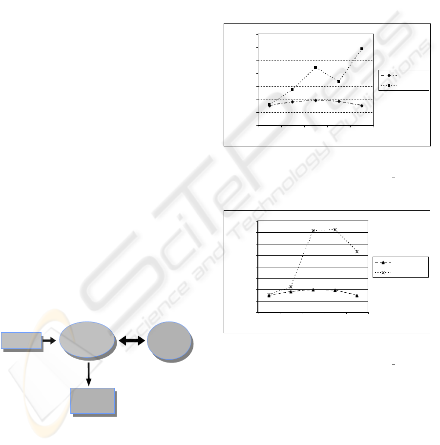
The results of makespan for small, medium and

large size Grids obtained with the hyper-heuristic are

compared with those of a random choice method (see

Figures 5 to 7). In these ﬁgures, the Y-axis indicates

the makespan value (in arbitrary time units) and the

X-axis the immediate vs batch ratio used.

2000000

4000000

6000000

8000000

10000000

12000000

14000000

0.00 0.25 0.50 0.75 1.00

Small

Small_RND

Figure 5: Comparison of makespan values for the dynamic

environment (small size grid) obtained with the hyper-

heuristic and a random choice method (denoted

RND

2000000

4000000

6000000

8000000

10000000

12000000

14000000

16000000

0.00 0.25 0.50 0.75 1.00

Medium

Medium_RND

Figure 6: Comparison of makespan values for the dynamic

environment (medium size grid) obtained with the hyper-

heuristic and a random choice method (denoted

RND

5.1 Evaluation

From the results of static setting (see Figures 1 to 3)

we can observe that the ad hoc methods perform quite

differently on the set of considered static instances.

On the other hand, it can also be observed that, their

performance depends on the objective to optimize.

Thus, for instance, MCT performs well for optimizing

makespan but very bad for optimizing ﬂowtime. As a

matter of fact, these results were the starting point to

ICSOFT 2007 - International Conference on Software and Data Technologies

134

5000000

10000000

15000000

20000000

25000000

30000000

35000000

0.00 0.25 0.50 0.75 1.00

Immediate vs Batch ratio

Makespan (miillisecs)

Large

Large_RND

Figure 7: Comparison of makespan values for the dynamic

environment (large size grid) obtained with the hyper-

heuristic and a random choice method (denoted

RND

study the performance of the hyper-heuristic using a

Grid simulator. On the dynamic setting (see Figures 5

to 7) we clearly see that the hyper-heuristic produces

high quality planning of jobs as compared to pure ran-

dom choices of ad hoc methods.

6 CONCLUSION AND FUTURE

WORK

In this work we have presented an hyper-heuristic

that uses a set of parameters and ad hoc methods for

scheduling independent jobs to Grid resources. The

hyper-heuristic tries to deduce the Grid resources and

jobs characteristics and applies the ad hoc method

that yield the best planning of jobs for the Grid con-

ﬁguration.

From the experimental evaluation, we observed

that the planning of jobs to grid resources obtained by

the hyper-heuristic using guided decisions are much

better and coherent than pure random decisions (with-

out any knowledge of the underlaying Grid charac-

teristics). For makespan, we have seen that the re-

sults worsen when the ratio of immediate/batch jobs

is close to 0.5, which is an indicator that immediate

and batch methods “damage” each others strategy. On

the other hand, for ﬂowtime, when the ratio of im-

mediate/batch is favorable to batch, better results are

obtained.

We plan to evaluate the hyper-heuristic in a real

grid, on the one hand by developing an interface to

use it, and on the other, by incorporating a module

that will be in charge of extracting the state of the net

(grid characteristics, job characteristics etc.) and will

pass it to the hyper-heuristic.

ACKNOWLEDGEMENTS

This research is partially supported by Projects

ASCE TIN2005-09198-C02-02, FP6-2004-ISO-

FETPI (AEOLUS) and MEC TIN2005-25859-E.

REFERENCES

Abraham, A., Buyya, R., and Nath, B. (2000). Nature’s

heuristics for scheduling jobs on computational grids.

In The 8th IEEE International Conference on Ad-

vanced Computing and Communications, India.

Braun, T., Siegel, H., Beck, N., Boloni, L., Maheswaran,

M., Reuther, A., Robertson, J., Theys, M., and Yao,

B. (2001). A comparison of eleven static heuristics

for mapping a class of independent tasks onto hetero-

geneous distributed computing systems. Journal of

Parallel and Distributed Computing, 61(6):810–837.

Casanova, H. and Dongarra, J. (1998). Netsolve: Network

enabled solvers. IEEE Computational Science and

Engineering, 5(3):57–67.

Foster, I. and Kesselman, C. (1998). The Grid - Blueprint

for a New Computing Infrastructure. Morgan Pub.

Foster, I., Kesselman, C., and Tuecke, S. (2001). The

anatomy of the grid. International Journal of Super-

computer Applications, 15(3).

Garey, M. and Johnson, D. (1979). Computers and

Intractability – A Guide to the Theory of NP-

Completeness. W.H. Freeman and Co.

Linderoth, L. and Wright, S. (2003). Decomposition algo-

rithms for stochastic programming on a computational

grid. Computational Optimization and Applications,

24:207–250.

Maheswaran, M., Ali, S., Siegel, H., Hensgen, D., and Fre-

und, R. (1999). Dynamic mapping of a class of in-

dependent tasks onto heterogeneous computing sys-

tems. Journal of Parallel and Distributed Computing,

59(2):107–131.

Phatanapherom, S. and Kachitvichyanukul, V. (2003). Fast

simulation model for grid scheduling using hypersim.

In Proceedings of the 2003 Winter Simulation Confer-

ence, New Orleans, USA.

Wright, S. (2001). Solving optimization problems on com-

putational grids. Optima, 65.

Wu, M.-Y. and Shu, W. (2001). A high-performance map-

ping algorithm for heterogeneous computing systems.

In Proceedings of the 15th International Parallel &

Distributed Processing Symposium, page 74.

A HYPER-HEURISTIC FOR SCHEDULING INDEPENDENT JOBS IN COMPUTATIONAL GRIDS

135