
INCLUDING IMPROVEMENT OF THE EXECUTION TIME IN A
SOFTWARE ARCHITECTURE OF LIBRARIES WITH
SELF-OPTIMISATION
Luis-Pedro Garc
´
ıa
Servicio de Apoyo a la Investigaci
´
on Tecnol
´
ogica, Universidad Polit
´
ecnica de Cartagena, 30203 Cartagena, Spain
Javier Cuenca
Departamento de Ingenier
´
ıa y Tecnolog
´
ıa de Computadores, Universidad de Murcia, 30071 Murcia, Spain
Domingo Gim
´
enez
Departamento de Inform
´
atica y Sistemas Inform
´
aticos, Universidad de Murcia, 30071 Murcia, Spain
Keywords:
Auto-tuning, performance modelling, self-optimisation, hierarchy of libraries.
Abstract:
The design of hierarchies of libraries helps to obtain modular and efficient sets of routines to solve problems
of specific fields. An example is ScaLAPACK’s hierarchy in the field of parallel linear algebra. To facilitate
the efficient execution of these routines, the inclusion of self-optimization techniques in the hierarchy has been
analysed. The routines at a level of the hierarchy use information generated by routines from lower levels. But
sometimes, the information generated at one level is not accurate enough to be used satisfactorily at higher
levels, and a remodelling of the routines is necessary. A remodelling phase is proposed and analysed with a
Strassen matrix multiplication.
1 INTRODUCTION
Important tuning systems exists that attempt to adapt
software to tune automatically to the conditions of the
execution platform. These include FFTW for discrete
Fourier transforms (Frigo, 1998), ATLAS (Whaley
et al., 2001) for the BLAS kernel, sparsity (Dongarra
and Eijkhout, 2002) and (Vuduc et al., 2001), SPI-
RAL (Singer and Veloso, 2000) for signal and image
processing, MPI collective communications (Vadhi-
yar et al., 2000), linear algebra routines (Chen. et al.,
2004) and (Katagiri et al., 2005), etc. Furthermore,
the development of automatically tuned software fa-
cilitates the efficient utilisation of the routines by non-
expert users. For any tuning system, the main goal is
to minimise the execution time of the routine to tune,
but with the important restriction of not increasing the
installation time of that routine too much.
A number of auto-tuning approaches are focused
on modelling the execution time of the routine to op-
timise. When the model has been obtained theoreti-
cally and/or experimentally, given a problem size and
execution environment, this model is used to obtain
the values of some adjustable parameters with which
to minimise the execution time. The approach chosen
by FAST (Caron et al., 2005) is an extensive bench-
mark followed by a polynomial regression applied to
find optimal parameters for different routines. (Vuduc
et al., 2001) apply the polynomial regression in their
methodology to decide the most appropriate version
from variants of a routine. They also introduce a
black-box pruning method to reduce the enormous
implementation spaces. In the approach of FIBER
(Katagiri et al., 2003) the execution time of a routine
is approximated by fixing one parameter and varying
the other. A set of polynomial functions of grades 1
to 5 are generated and then the best one is selected.
The values provided by these functions for differ-
ent problem sizes are used to generate other function
where now the second parameter is fixed and the first
one is varied. (Tanaka et al., 2006) introduce a new
method, named Incremental Performance Parameter
Estimation, in which the estimation of the theoretical
model by polynomial regression is started from the
least sampling points and incremented dynamically to
improve accuracy. Initially, they apply it on sequen-
156
García L., Cuenca J. and Giménez D. (2007).
INCLUDING IMPROVEMENT OF THE EXECUTION TIME IN A SOFTWARE ARCHITECTURE OF LIBRARIES WITH SELF-OPTIMISATION.
In Proceedings of the Second International Conference on Software and Data Technologies - SE, pages 156-161
DOI: 10.5220/0001337501560161
Copyright
c
SciTePress
tial platforms and with just one algorithmic parameter
to seek. (Lastovetsky et al., 2006) reduce the num-
ber of sampling points starting from a previous shape
of the curve that represents the execution time. They
also introduce the concept ”speed band” as the natural
way to represent the inherent fluctuations in the speed
due to changes in load over time.
In this context, our approach has used dense lin-
ear algebra software for message-passing systems as
routines to be tuned. In our previous studies (Cuenca
et al., 2004) a hierarchical approach to performance
modelling was proposed. The basic idea has been to
exploit the natural hierarchy existing in linear alge-
bra programs. The execution time models of lower-
level routines are constructed firstly from code anal-
ysis. After that, to model a higher-level routine, the
execution time is estimated by injecting in its model
the information of those lower-level routines that are
invoked by the higher-level routine.
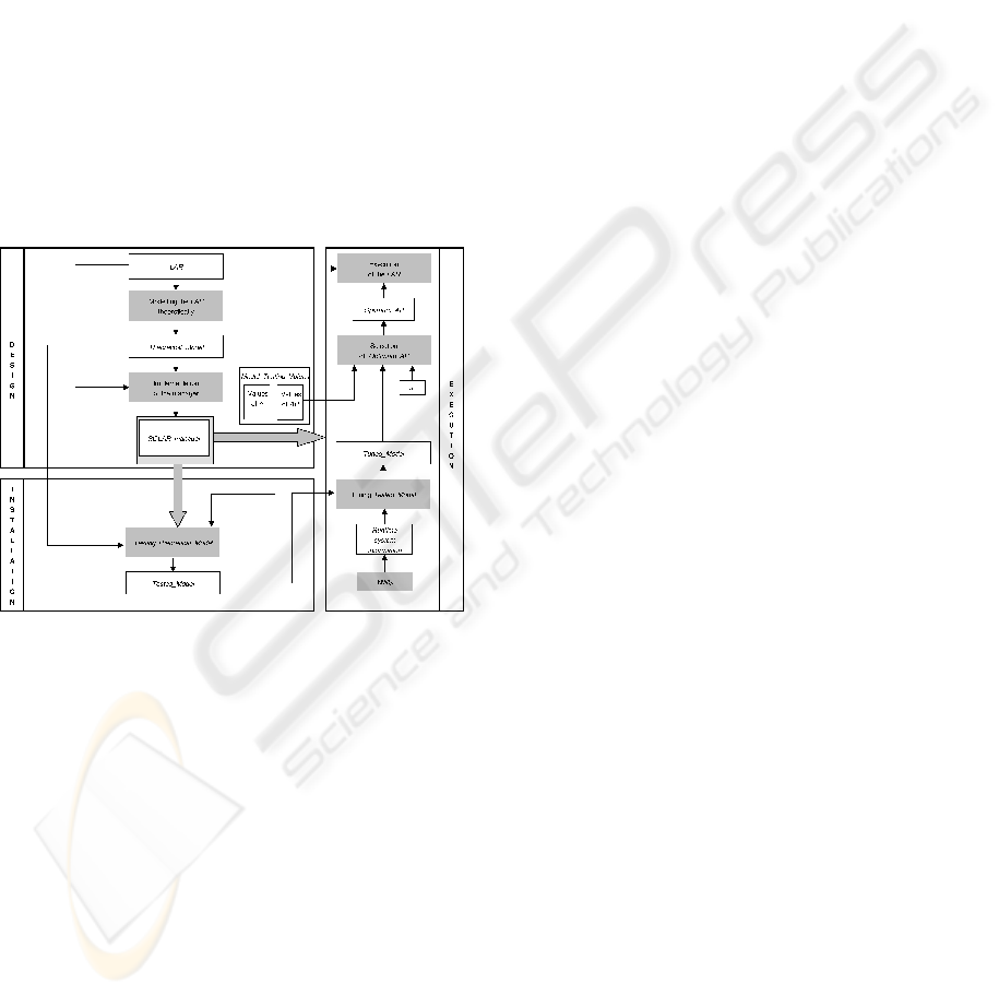
Figure 1: Life-cycle of a SOLAR.
In this work, a technique for redesigning the
model from a serial of sampling points by means of
polynomial regression has been included in our orig-
inal methodology. The basic idea is to start from the
hierarchical model using the information from lower
level routines to model the higher level ones without
experimenting with these. However, if for a concrete
routine all this information is not useful enough, then
its model would be built again from the beginning us-
ing a series of experimental executions and polyno-
mial regression applied appropriately.
The rest of the paper is organised as follows:
in section 2 the improved architecture of a self-
optimised routine is analysed, then in section 3 some
experimental results are described with their special
features, and finally, in section 4 the conclusions are
summarised and possible future research is outlined.
2 CREATION AND UTILISATION
OF A SELF-OPTIMISED
LINEAR ALGEBRA ROUTINE
In this section the design, installation and execution of
a Self-Optimised Linear Algebra Routine (SOLAR) is
described step by step, following the scheme in fig-
ure 1. This life-cycle of a routine such as is described
bellow is a modification/extension of that originally
proposed in (Cuenca et al., 2004). The main differ-
ence lies in that in our previous work, during the in-
stallation of a routine its theoretical model and infor-
mation from lower level routines were used to com-
plete a theoretical-practical model. Now this process
is extended with a testing sub-phase of this model,
comparing from a series of sampling points (different
sets of problem sizes plus algorithmic parameters) the
distance between the modelled time and the experi-
mental one. If this distance is not small enough then
a remodelling sub-phase starts, where a new model
of the routine is built from zero, using benchmarking
and polynomial regression in different ways.
2.1 Design
This process is performed only once by the designer
of the Linear Algebra Routine (LAR), when this LAR
is being created. The tasks to be done are:
Create the LAR: The LAR is designed and pro-
grammed if it is new. Otherwise, the code of the LAR
does not have to be changed.
Model the LAR theoretically: The complexity of
the LAR is studied, obtaining an analytical model of
its execution time as a function of the problem size,
n, the System Parameters (SP) and the Algorithmic
Parameters (AP): T
exec
= f(SP, AP, n).
SP describe how the hardware and the lower level
routines affect the execution time of the LAR. SP
are costs of performing arithmetic operations by us-
ing lower level routines, for example, BLAS routines
(Dongarra et al., 1988); and communication parame-
ters (start-up, t
s
, and word-sending time, t
w
).
AP represent the possible decisions to take in or-
der to execute the LAR. These are the block size, b, in
block based algorithms, and parameters defining the
logical topology of the processes grid or the data dis-
tribution in parallel algorithms.
Select the parameters for testing the model:
The most significant values of n and AP are provided
by the LAR designer. They will be used to test the the-
oretical model during the installation process. These
AP values will also be used at execution time to se-
lect their theoretical optimum values when the run-
time problem size is known.
INCLUDING IMPROVEMENT OF THE EXECUTION TIME IN A SOFTWARE ARCHITECTURE OF LIBRARIES
WITH SELF-OPTIMISATION
157

Create the SOLAR manager: The
SOLAR
manager is also programmed by the LAR
designer. This subroutine is the engine of the SOLAR.
It is in charge of managing all the information inside
this software architecture. At installation time, it tests
the theoretical model and, if necessary, improves it.
At execution time, it tunes the model according to
the situation of the platform. Then, using the tuned
model, it decides the appropriate values for the AP,
and finally calls the LAR.
2.2 Installation
In the installation process of a SOLAR the tasks per-
formed by the SOLAR
manager are:
Execute the LAR: The LAR is executed using the
different values of n and AP contained in the structure
Model
Testing Values.
Test the model: The obtained execution times are
compared with the theoretical times provided by the
model for the same values of n and AP, and using the
SP values returned by the previously installed lower
level SOLARs
1
. If the averaged distance between the-
oretical and experimental times exceed an error quota,
the SOLAR
manager would remodel the LAR.
2.2.1 Remodelling the LAR
If the installation process reaches this step, is because
the information of the SP obtained from lower level
SOLARs has not been accurate enough for the cur-
rent SOLAR model, and so the SOLAR
manager has
to build an improved model by itself.
This new model is built, from the original model
by designing a polynomial scheme for the different
combinations of n and AP in Model
Testing Values.
The coefficients of each term of this polynomial
scheme must be calculated. In order to determine
these coefficients, four different methods could be
applied in the following order: FIxed Minimal Exe-
cutions (FI-ME), VAriable Minimal Executions (VA-
ME), FIxed Least Square (FI-LS) and VAriable Least
Square (VA-LS). When one of them provides enough
accuracy then the other methods are not used.
FI-ME: The experimental time function is ap-
proximated by a single polynomial. The coefficients
are obtained with the minimum number of executions
needed.
VA-ME: The experimental time function is ap-
proximated by a set of p polynomials corresponding
1
When a SOLAR receives a request from an upper level
SOLAR about its execution time for a specific combination
of (n, AP) it substitutes these values in its tested model, ob-
taining the corresponding theoretical time, which it sends
back to the SOLAR in question.
to p intervals of combinations of (n, AP). For each of
these intervals the above method is applied.
FI-LS: In this method, like in the FI-ME method,
the experimental time function is approximated by a
single polynomial. Now a least square method that
minimises the distance between the experimental and
the theoretical time for a number of combinations of
(n, AP) is applied to obtain the coefficients.
VA-LS: As in the VA-ME method, the execution
time function is divided in p intervals, applying the
FI-LS method in each one.
2.3 Execution
When a SOLAR is called to solve a problem of size
n
R
, the following tasks are carried out:
Collecting system information: The
SOLAR
manager collects the information that
the NWS (Wolski et al., 1999) (or any other similar
tool installed on the platform) provides about the
current state of the system (CPU load and network
load between each pair of nodes).
Tuning the model: The SOLAR
manager tunes
the Tested
Model according to the system condi-
tions. Basically the arithmetic parts of the model will
change inversely to the availability of the CPU, and
the same occurs for the communication parts of the
model and the availability of the network.
Selection of the Optimum
AP: Using the
Tuned
Model, with n = n
R
, the SOLAR manager
looks for the combination of AP values that provides
the lowest execution time.
Execution of the LAR: Finally, the
SOLAR
manager calls the LAR with the param-
eters (n
R
, Optimum
AP).
3 SELF-OPTIMISED LINEAR
ALGEBRA ROUTINE SAMPLES
In this section the indicated procedure in 2 is ap-
plied to the Strassen algorithm. The idea is to show,
through this particular application, that it is possible
to automatically obtain the best possible execution
time for given input parameters (n, AP), as well as
the scheme followed by a SOLAR
manager to build
(if necessary) a new model for a LAR.
3.1 Strassen Matrix-Matrix
Multiplication
(Strassen, 1969) introduced an algorithm to multiply
matrices of n × n size which has a lower level com-
plexity than the classical O(n
3
). It is based on a
ICSOFT 2007 - International Conference on Software and Data Technologies
158

scheme for the product, C = AB, of two 2 × 2 block
matrices:
C
11
C
12
C
21
C
22
=
A
11
A
12
A
21
A
22
×
B
11
B
12
B
21
B
22
where each block is square. In the ordinary algo-
rithm there are eight multiplications and four addi-
tions. Strassen discovered that the original algorithm
can be reorganized to compute C with just seven mul-
tiplications and eighteen additions:
Pre-additions Recursive Calls
S
1
= A
11
+ A
22
T
1
= B
11
+ B
22
P
1
= S
1
× T
1
S
2
= A
21
+ A
22
T
2
= B
12
− B
22
P
2
= S
2
× B
11
S
3
= A
11
+ A
12
T
3
= B
21
− B
11
P
3
= A
11
× T
2
S
4
= A
21
− A
11
T
4
= B
11
+ B
12
P
4
= A
22
× T
3
S
5
= A
12
− A
22
T
5
= B
21
+ B
22
P
5
= S
3
× B
22
P
6
= S
4
× T
4
P
7
= S
5
× T
5
Post-additions
C
11
= P
1
+ P
4
− P
5
+ P
7
C
12
= P
3
+ P
5
C
21
= P
2
+ P
4
C
22
= P
1
+ P
3
− P
2
+ P
6
Strassen algorithm can apply to each of the half-size
block multiplications associated with P
i
. Thus, if
the original A and B are square matrices of dimen-
sion n = 2
q
, the algorithm can be applied recursively.
As a result, Strassen’s algorithm has a complexity of
O(n
log
2
7
) ≈ O(n
2.807
). Variations of this algorithm
available in the literature (Douglas et al., 1994) and
(Huss-Lederman et al., 1996), allow us to handle ma-
trices of arbitrary size.
In order to build the analytical model of the run
time, we identify different parts of the Strassen algo-
rithm with different basic routines:
• The BLAS3 function DGEMM is used to com-
pute the seven P
i
at the lower level. If the recur-
sion level used is l, the matrix multiplications are
made in blocks of size
n
2
l
.
• In the recursion level l, with l = 1, 2, 3, . . ., there
are 7
(l−1)
× 18 matrix additions of size
n
2
l
. The
BLAS1 function DAXPY can be used to compute
S
i
, T
i
and C
ij
.
The execution time for this algorithm can be mod-
elled by the formula:
T
S
= 7
l
t
mult
n
2
l
+ 18
l
∑
i=1
7
i−1
t
add
n
2
i
(1)
where t
mult
(
n
2
l
) is the theoretical execution time for
one matrix multiplication of size
n
2
l
, and t
add
(
n
2
i
) is
the theoretical execution time for a matrix addition of
size
n
2
i
.
3.2 Experimental Results
The experiments have been performed in two differ-
ent systems: a Linux Intel Xeon 3.0 GHz workstation
(Xeon) and a Unix HP-Alpha 1.0 GHz workstation
(Alpha). Optimized versions of BLAS (provided by
the manufactures) have been used for the basic rou-
tines. In both cases the experiments are repeated sev-
eral times, obtaining an average value.
In the experiments for Xeon and Alpha we found,
that for the matrix multiplication the third order poly-
nomial function was the best and for matrix addi-
tion the best was the sixth order polynomial function.
Therefore we use this number of coefficients for its
SOLAR. These coefficients can be calculated using
any of the four methods described in 2.2.1, but in
Xeon and Alpha good results were obtained using the
FI-LS method.
For Matrix Multiplication the values for the struc-
ture Model
Testing Values in Xeon and Alpha are:
Matrix sizes n =
{
500, 1000, 1500, 2000, . . . , 10000
}
;
and for Matrix Addition: Matrix sizes n =
{
64, 128, 192, 256, . . . , 2000
}
.
In Xeon the polynomial functions that model the
basic routines are:
• Matrix Multiplication: 1.338 × 10
−01
− 2.261 ×
10
−04
n+ 1.039× 10
−07
n
2
+ 3.963× 10
−10
n
3
.
• Matrix Addition: 1.507 × 10
−03
− 2.952 × 10
−05
n +
1.521 × 10
−07
n
2
− 1.970 × 10
−10
n
3
+ 1.614 ×
10
−13
n
4
− 6.367× 10
−17
n
5
+ 9.687× 10
−21
n
6
.
and in Alpha:
• Matrix Multiplication: −9.517 × 10
−02
+ 2.128 ×
10
−04
n− 9.079× 10
−08
n
2
+ 1.136× 10
−09
n
3
.
• Matrix Addition: −9.983× 10
−04
+ 1.683 × 10
−05
n−
6.700 × 10
−08
n
2
+ 1.624 × 10
−10
n
3
− 1.284 ×
10
−13
n
4
+ 4.698× 10
−17
n
5
− 6.509× 10
−21
n
6
.
The SOLAR
manager strassen uses the
theoretical model shown in equation 1, and
sends a request for the theoretical execution
time to the SOLAR
manager at lower levels:
SOLAR
manager mult and SOLAR manager add
for t
mult
(
n
2
l
) and t
add
(
n
2
i
) respectively. For the
Strassen algorithm the values for the structure
Model
Testing Values in Xeon and Alpha are:
l =
{
1, 2, 3
}
and n =
{
3072, 4096, 5120, 6144
}
For the SOLAR
manager to calculate
an error quota for the Theoretical
Model,
the function Φ
err
is defined: Φ
err
=
∑
Model
Testing Values
1−
Theoretical
Model
LAR Execution
× 100
INCLUDING IMPROVEMENT OF THE EXECUTION TIME IN A SOFTWARE ARCHITECTURE OF LIBRARIES
WITH SELF-OPTIMISATION
159

Table 1: Comparison between measured execution times (in
seconds) with modelled times for Strassen algorithm. In
Xeon and Alpha.
Xeon Alpha
n l
mod. exp. dev. mod. exp. dev.
(%) (%)
3072 1 11.75 12.86 8.58 29.96 29.70 0.89
3072 2
13.90 13.63 1.99 28.54 27.82 2.57
3072 3
37.04 15.76 135.06 17.55 27.61 36.46
4096 1 27.21 29.71 8.41 69.85 70.85 1.43
4096 2
28.59 30.10 5.02 66.04 64.55 2.30
4096 3
48.76 33.34 46.26 57.82 62.56 7.58
5120 1 53.14 56.83 6.51 135.03 134.67 0.26
5120 2
53.53 56.43 5.13 125.76 123.38 1.92
5120 3
71.08 60.19 18.09 118.12 118.45 0.28
6144 1 96.48 96.32 0.17 229.79 232.27 1.07
6144 2
95.39 93.69 1.82 211.10 210.88 0.11
6144 3
110.40 98.39 12.21 201.15 199.33 0.92
Table 1 shows the theoretical execution time pro-
vided by the model (mod.), the experimental execu-
tion time (exp.) and the deviation (dev.) (
|t
mod
−t
exp
|
t
exp
)
for the values in Model
Testing Values. The op-
timum experimental and theoretical times are high-
lighted. In Xeon and Alpha the SOLAR
Manager
makes a correct prediction of the level of recursion
with which the optimal execution times are obtained.
Only in Xeon and for matrix size 5120 the recursion
levels are different. In this case the execution time
obtained with the values provided by the model is
about 0.71% higher than the optimum experimental
time. The deviation, however, ranged from 0.17 %
to 135.06 % in Xeon and from 0.11 % to 36.46 %
in Alpha, and the fluctuation is large; Φ
err
= 8.38 %
for Xeon and Φ
err
= 0.87 % for Alpha. This means
that the SOLAR
manager has to build an improved
model by itself for Xeon. In Alpha it is not neces-
sary to make a remodelling of the LAR, and so the
Theoretical
Model would be the Tested Model.
3.2.1 Remodelling Strassen
In Xeon it is necessary to build a new model for the
Strassen algorithm. The scheme consists of defining
a set of third grade polynomial functions from the
Strassen’s theoretical model. This set of polynomials
is:
T
S
(n, l) = 2× 7
l
n
2
l
3
M(l) +
18
4
n
2
A(l)
l
∑
i=1
7
4
i−1
(2)
where the coefficients M(l) and A(l) must be calcu-
lated. The parameter l (recursion level) is fixed and
the problem size n varies. For each l a set of Strassen
executions is carried out, and the values M(l) and A(l)
are obtained using the least squares method (FI-LS).
Table 2 shows the values obtained for M(l)
and A(l) in Xeon with l =
{
1, 2, 3, 4
}
and n =
{
512, 1024, 1536, 2048, 2560, 3072, 3584, 4096, 4608
}
.
Table 2: Values of M(l) and A(l) in Xeon.
l M(l) A(l)
1 2.222× 10
−10
3.890× 10
−08
2 2.244× 10
−10
3.033× 10
−08
3 1.986× 10
−10
3.025× 10
−08
4 3.477× 10
−10
1.528× 10
−08
The A(l) values can be approximated by a first
grade polynomial and the M(l) values by a second
grade polynomial. The coefficients are obtained by
least squares. Finally, the formulae for M(l) and A(l)
are:
• M(l) = 1.907 × 10
−10
+ 4.580 × 10
−11
× l − 1.445 ×
10
−11
× l
2
.
• A(l) = 4.378× 10
−08
− 5.131× 10
−09
× l.
Thus, we have a single theoretical model for any
combination of (n, AP).
Now SOLAR
manager strassen verifies the new
Theoretical
Model for the Strassen algorithm. The
values for the structure Model
Testing Values are l =
{
1, 2, 3
}
and n =
{
2688, 3200, 5120, 5632
}
In the table 3 it is seen that the model success-
fully predicts the recursion level with which the opti-
mum execution times are obtained, except for matrix
size 5120. In this case the execution time obtained
with the values provided by the model is about 3.49 %
higher than the optimum experimental time. The rela-
tive error ranges from 0.17 % to 15.52 % and the fluc-
tuation is smaller, Φ
err
= 0.37 %. This means that the
new Theoretical
Model will be the Tested Model.
Table 3: Comparison of the experimental execution times
(in seconds) with modelled times for Strassen algorithm
with remodelling. In Xeon.
n l mod. exp. dev. (%)
2688 1 7.87 8.80 11.92
2688 2 8.40 9.67 15.23
2688 3 10.28 10.52 2.38
3200 1 13.02 14.51 11.92
3200 2 13.56 15.51 14.38
3200 3 16.00 16.30 1.87
5120 1 56.80 56.71 0.17
5120 2 56.44 57.01 1.00
5120 3 60.04 55.09 8.25
5632 1 75.78 74.92 1.12
5632 2 73.50 74.56 1.45
5632 3 71.70 70.97 1.03
The values of the algorithmic parameters vary for
different systems and problem sizes, but with the
ICSOFT 2007 - International Conference on Software and Data Technologies
160

model and with the inclusion of the possibility of re-
modelling, a satisfactory selection of the parameters
is made in all the cases, enabling us to take the appro-
priate decisions about their values prior to the execu-
tion.
4 CONCLUSIONS AND FUTURE
WORKS
The use of modelling techniques can contribute to im-
prove the decisions taken in order to reduce the execu-
tion time of the routines. The modelling allows us to
introduce information about the behavior of the rou-
tine in the tuning process, guiding this process.
It is necessary that the modelling time is small be-
cause at least part of this process could be carried out
in each installation of the routines. Therefore, differ-
ent ways of reducing it have been studied here, and
the results have been satisfactory.
Today, our research group is working on the inclu-
sion of meta-heuristics techniques in the modelling
(Mart
´
ınez-Gallar et al., 2006), and in applying the
same methodology to other types of routines and al-
gorithmic schemes (Cuenca et al., 2005) and (Carmo-
Boratto et al., 2006).
ACKNOWLEDGEMENTS
This work partially has been supported by the Conse-
jer
´
ıa de Educaci
´
on de la Regi
´
on de Murcia, Fundaci
´
on
S
´
eneca 02973/PI/05.
REFERENCES
Carmo-Boratto, M. D., Gim
´
enez, D., and Vidal, A. M.
(2006). Automatic parametrization on divide-and-
conquer algorithms. In proceedings of International
Congress of Mathematicians.
Caron, E., Desprez, F., and Suter, F. (2005). Parallel exten-
sion of a dynamic performance forecasting tool. Scal-
able Computing: Practice and Experience, 6(1):57–
69.
Chen., Z., Dongarra, J., Luszczek, P., and Roche, K. (2004).
LAPACK for clusters project: An example of self
adapting numerical software. In proceedings of the
HICSS 04’, page 90282.1.
Cuenca, J., Gim
´
enez, D., and Gonz
´
alez, J. (2004). Archi-
tecture of an automatic tuned linear algebra library.
Parallel Computing, 30(2):187–220.
Cuenca, J., Gim
´
enez, D., and Mart
´
ınez-Gallar, J. P. (2005).
Heuristics for work distribution of a homogeneous
parallel dynamic programming scheme on heteroge-
neous systems. Parallel Computing, 31:735–771.
Dongarra, J., Croz, J. D., and Duff, I. S. (1988). A set of
level 3 basic linear algebra subprograms. ACM Trans.
Math. Software, 14:1–17.
Dongarra, J. and Eijkhout, V. (2002). Self-adapting numer-
ical software for next generation applications. In ICL
Technical Report, ICL-UT-02-07.
Douglas, C. C., Heroux, M., Slishman, G., and Smith, R. M.
(1994). GEMMW: A portable level 3 BLAS Wino-
grad variant of Strassen’s matrix–matrix multiply al-
gorithm. J. Comp. Phys., 110:1–10.
Frigo, M. (1998). FFTW: An adaptive software architecture
for the FFT. In proceedings of the ICASSP conference,
volume 3, pages 1381–1384.
Huss-Lederman, S., Jacobson, E. M., Tsao, A., Turnbull,
T., and Johnson, J. R. (1996). Implementation of
strassen’s algorithm for matrix multiplication. In pro-
ceedings of Supercomputing ’96, page 32.
Katagiri, T., Kise, K., Honda, H., and Yuba, T. (2003).
FIBER: A generalized framework for auto-tuning
software. Springer LNCS, 2858:146–159.
Katagiri, T., Kise, K., Honda, H., and Yuba, T. (2005). AB-
CLib
DRSSED: A parallel eigensolver with an auto-
tuning facility. Parallel Computing, 32:231–250.
Lastovetsky, A., Reddy, R., and Higgins, R. (2006). Build-
ing the functional performance model of a processor.
In proceedings of the SAC’06, pages 23–27.
Mart
´
ınez-Gallar, J. P., Almeida, F., and Gim
´
enez, D. (2006).
Mapping in heterogeneous systems with heuristical
methods. In proceedings of PARA’06.
Singer, B. and Veloso, M. (2000). Learning to predict per-
formance from formula modeling and training data.
In proceedings of the 17th International Conference
on Mach. Learn., pages 887–894.
Strassen, V. (1969). Gaussian elimination is not optimal.
Numerische Mathematik, 3(14):354–356.
Tanaka, T., Katagiri, T., and Yuba, T. (2006). d-spline based
incremental parameter estimation in automatic perfor-
mance tuning. In proceedings of the PARA’06.
Vadhiyar, S. S., Fagg, G. E., and Dongarra, J. J. (2000). Au-
tomatically tuned collective operations. In proceed-
ings of Supercomputing 2000, pages 3–13.
Vuduc, R., Demmel, J. W., and Bilmes, J. (2001). Statistical
models for automatic performance tuning. In proceed-
ings of ICCS’01, LNCS, volume 2073, pages 117–126.
Whaley, R. C., Petitet, A., and Dongarra, J. J. (2001). Au-
tomated empirical optimizations of software and the
ATLAS project. Parallel Computing, 27(1-2):3–35.
Wolski, R., Spring, N. T., and Hayes, J. (1999). The net-
work weather sevice: a distributed resource perfor-
mance forescasting service for metacomputing. Jour-
nal of Future Generation Computing System, 15(5–
6):757–768.
INCLUDING IMPROVEMENT OF THE EXECUTION TIME IN A SOFTWARE ARCHITECTURE OF LIBRARIES
WITH SELF-OPTIMISATION
161
