OPTIMIZATION OF DISTRIBUTED OLAP CUBES WITH AN

ADAPTIVE SIMULATED ANNEALING ALGORITHM

Jorge Loureiro

Departamento de Informática, Escola Superior de Tecnologia de Viseu

Instituto Superior Politécnico de Viseu, Campus Polit

écnico de Repeses, 3505-510 Viseu, Portugal

Orlando Belo

Departamento de Informática, Escola de Engenharia

Universidade do Minho, Campus de Gualtar, 4710-057 Braga, Portugal

Keywords: Distributed Data Cube Selection, Adaptive Simulated Annealing Algorithm, Multi-Node OLAP Systems

Optimization.

Abstract: The materialization of multidimensional structur

es is a sine qua non condition of performance for OLAP

systems. Several proposals have addressed the problem of selecting the optimal set of aggregations for the

centralized OLAP approach. But the OLAP structures may also be distributed to capture the known

advantages of distributed databases. However, this approach introduces another term into the optimizing

equation: space, which generates new inter-node subcubes’ dependencies. The problem to solve is the

selection of the most appropriate cubes, but also its correct allocation. The optimizing heuristics face now

with extra complexity, hardening its searching for solutions. To address this extended problem, this paper

proposes a simulated annealing heuristic, which includes an adaptive mechanism, concerning the size of

each move of the hill climber. The results of the experimental simulation show that this algorithm is a good

solution for this kind of problem, especially when it comes to its remarkable scalability.

1 INTRODUCTION

The multidimensional vision, a main characteristic

of On-Line Analytical Processing (OLAP) systems,

makes their success. But the increasing complexity

and size of the multidimensional structures, denoted

as materialized views or subcubes, the support of a

fast query answering, independently of the

aggregation level of the required information, imply

new approaches to their optimization, beyond the

classical cube selection solutions, e.g. (Harinarayan

et al., 1996), (Gupta & Mumick, 1999), (Liang et al.

2001), using greedy heuristics, (Zhang et al., 2001),

(Lin & Kuo, 2004), using genetic approaches or in

(Kalnis et al. 2002), using randomized approaches.

One of the new solutions is the distribution of the

materialized subcubes, aiming to capture the known

advantages of database distribution: a sustained

growth of processing capacity (easy scalability)

without an exponential increase of costs, and an

increased availability of the system, as it eliminates

the dependence from a single source and avoids

bottlenecks. This distribution may be achieved in

different ways; in this paper, we focus in one of

them: distributing the OLAP cube by several nodes,

inhabiting in close or remote sites, interconnected by

communication links, generating a multi-node

OLAP approach (M-OLAP). The traditional cube

selection problem (the materialization of only the

most beneficial subcubes) is now extended, as we

have a new dimension: space. It’s not enough to

select the most beneficial subcubes; they also have

to be conveniently located. In the distributed

scenery, we have n storage and processing nodes,

named OLAP server nodes (OSN), with a known

processing power and storage space, interconnected

by a network, being able to share data or redirecting

queries to other nodes.

The authors in (Bauer & Lehn

er, 2003)

introduced the distributed aggregation lattice and

proposed a distributed node set greedy algorithm

that addressed the distributed view selection

Loureiro J. and Belo O. (2007).

OPTIMIZATION OF DISTRIBUTED OLAP CUBES WITH AN ADAPTIVE SIMULATED ANNEALING ALGORITHM.

In Proceedings of the Second International Conference on Software and Data Technologies - Volume ISDM/WsEHST/DC, pages 21-28

DOI: 10.5220/0001342800210028

 SciTePress

problem, being shown that this algorithm has a

superior performance than the corresponding

standard greedy algorithm, using a benefit per unit

space metric. But they didn’t include maintenance

costs into the general optimization cost goal and also

didn’t include communication and node processing

power parameters into the cost formulas. This

distributed lattice framework is used in (Loureiro &

Belo, 2006a), but including real communication cost

parameters and processing node power, which led to

heterogeneity in the nodes and the network. To this

modified model, several estimation cost algorithms

were proposed (Loureiro & Belo, 2006a), (Loureiro

& Belo, 2006b), which used the intrinsic parallel

nature of the distributed OLAP architecture and time

as the cost unit. Framed on this model, in (Loureiro

& Belo, 2006c), a genetic co-evolutionary approach

is applied to the selection and allocation of cubes in

M-OLAP systems, where the genotype of each

specie is mapped to the subcubes to materialize in

each node. This problem is also addressed in

(Loureiro & Belo, 2006d), using another heuristic:

discrete particle swarm optimization. Globally, the

reported tests’ results show that both genetic

(especially in its co-evolutionary version) and

swarm approaches (both normal and cooperative

versions) have low complexity (lower for the normal

Di-PSO), being shown that they have a good

scalability, supporting easily an M-OLAP

architecture with several nodes and also suited for

moderate OLAP dimensionalities. Now, we use a

simulated annealing meta-heuristic to this same

problem, but using a more comprehensive cost

model, that introduces non-linearities, a better

support to maintenance cost estimation and different

algorithms to estimate the costs, which include the

use of a pipelining approach to simulate the parallel

tasks’ execution (Loureiro & Belo, 2006b). This

new approach is expected to have a good scalability,

regarding the results referred in (Kalnis et al. 2002),

which also will be welcome in M-OLAP

architectures.

2 HILL CLIMBING WITH

SIMULATED ANNEALING

The hill climbing heuristic is simple: a hill climber

moves randomly through the search space, trying to

find good solutions to the problem, restricted only

by constraints that may be imposed to the optimizing

process. This heuristic may be improved only

allowing moves (

) which improve the quality

of the solution. This is called iterative improvement

or local search. But if the hill climber falls into a

local optimum, it cannot escape from there, and the

search process ends abruptly. In (Kirkpatrick et al.,

1983) a simulated annealing meta-heuristic able to

solve this problem was proposed: the hill climber

could move to a worst place, jumping then out of the

local minimum. This trick is good, but must be

restricted, including an adaptive probabilistic

mechanism: the probability of accepting “bad”

moves (

−

) decreases with the on-going process.

The annealing schema explores the thermodynamic

analogy of the cooling of a melted solid: T (the

temperature) controls the probability of accepting

−

moves (and its extent). A simplified version of

the simulated annealing algorithm is shown in

Algorithm 1. As we can see, T (temperature) is a

parameter that controls the possibility of allowing

movements which degrade the solution. As Δ is the

loss of solution’s quality (in terms of the objective

function ), if Δ < 0, the new position is accepted

(the referred local search heuristic), but with a

probability

a movement with Δ > 0 (a

−Δ

−

move) will be possible, allowing the hill climber to

escape from local optima.

This probability has two immediate

consequences:

− Movements which imply low values of delta will

be admitted more often than the opposite: jumps

that imply a great loss in the solution’s quality

will have a low probability of happening.

− The value of T will be a factor which controls this

probability. Its value controls the exploration

versus exploitation trade-off: for the same delta’s

value, a high T implies a higher probability of

accepting moves which imply a higher

degradation of the quality’s solution (accepting

worst moves) and conversely.

Simulated Annealing Meta-Heuristic

Select a initial solution and an initial temperature

Begin

←

best

While not achieved stop criterion

←

solution in the neighbourhood of

←−() (')fs fs

// f(s) defines the quality of s

then

←

// the new solution is better

−Δ

else if

> rnd[0,1) then

← '

then

>() ( )

best

←

best

TT*

←

WhileEnd

Return

best

End

Algorithm 1: Simulated annealing meta-heuristic.

ICSOFT 2007 - International Conference on Software and Data Technologies

This way, a high initial T value allows the hill

climber to escape from local o

ptima. However, if T

remains the same for all the search process, the algorithm

will keep the exploration, without seeking for a deep

inspection in a particular region, what would be achieved

if the probability of accepting

−

moves was low. We

face then with two conflicting objectives. But if T had

initially a high value which would decrease until a low

value, the algorithm would have an initial phase where the

exploration was favored, being the situation reversed at

the end of the process, where almost (or even only) the

exploitation was allowed. In fact, as T decreases with the

iteration’s number, when T approaches zero, the

probability of accepting

−

moves almost reaches 0:

. Summarizing, T is set at an initial

high value T

−Δ

→⇒ →0

. After a pre-defined iterations’ number, it is

reduced by an

factor,

1nn

−

, being

←

Other cooling mechanisms were possible, e.g. 1)

decreasing T by a constant value, after a pre-defined

number of iterations or 2) even the decreasing value could

be successively lower as the end of the search process

approached.

3 PROBLEM DEFINITION AND

ALGORITHM’S APPLYING

The problem that we must solve may be defined like

this:

Definition 1: Selection and allocation of

distributed M problem. Let Q={q

, …, q

} be a set of

queries with access frequencies {fq

, …, fq

}, query

extension {qe

,…,qe

}; let update frequency and

extension be {fu

, …, fu

} and {ue

,…,ue

respectively, and let S

be the amount of

materializing space by OLAP node i. A solution to

the selection and allocation problem is a set of

subcubes M={s

,…,s

} with a constraint,

where

is the materializing space of all subcubes S

in node

, so that the total costs of answering all queries Q

and maintaining M, Cq(Q, M)+Cm(M) are minimal.

To use the simulated annealing meta-heuristic we

must, as we can see, referring to Algorithm 1:

1. find a way to code the problem;

2. generate the initial position of all hill climbers;

3. define the neighborhood of any position s;

4. define the hill climber’s movement scheme;

5. know how to evaluate the quality of each

solution (delta computing);

6. define and

(or any other cooling

mechanism).

Figure 1 shows a functional presentation of Hill

Climber with Simulated Annealing M-OLAP (HC-

SA M-OLAP) algorithm.

Concerning to the first referred issue, as we have

a space paradigm of the solutions, we must map

each possible M into the position of a hill climber.

As M may have a maximal number of subcubes

nS=n.Ls (where n is the number of OSNs and Ls is

the number of subcubes into the lattice), we must

have a multidimensional space of d=nS dimensions,

being each dimension mapped to a possible subcube

in M (in right lower corner of Figure 1, we have

shown the multidimensional space for a node with 8

possible subcubes). A position=1 for a dimension d

means that the corresponding subcube in M is

materialized and conversely. E.g., in Figure 1,

subcube S0 is mapped into the X dimension: as S0 is

materialized, the HC is at a 1 position. Summarizing,

as the search space has d dimensions, the position of

the hill climber is coded by a binary string where

each bit is then mapped to a subcube that may be (or

not) materialized into each node.

Relating to the second issue, as for the

generation of the initial genome in genetic

algorithms or the generation of the initial position of

a particle in particle swarm algorithms that we tested

in other research works, we opted for the random

generation of the initial position of each hill climber.

Concerning to the definition of the neighborhood

of a given position, as , any other

sM=

''sMM

≠ will be a new solution in the ’s

neighborhood. We may define a maximal Hamming

distance, mhd, which will limit the range of the

move of each step for any hill climber. Viewing this

scheme under the spatial paradigm, this will imply

that each journey of the HC is limited to a given

maximal range. In terms of the problem to solve, this

implies that the number of subcubes to dematerialize

or materialize in each iteration is limited and may be

changed, by specifying a different value.

The forth item, the hill climber’s movement

scheme (shown in the second round cornered

rectangle of Figure 1), is directly related to the

former definition of neighborhood: in each iteration

the dematerialization of dsc subcubes is allowed,

min

, as is the rematerialization of rsc

subcubes

min max

rdh rsc rdh

max

ddh dsc ddh≤≤

≤

, selecting both values

randomly inside the specified interval. Once again,

the balance of the relation exploration versus

exploitation is changed along the search process, by

decreasing dsc and rsc range (at each fudri – update

frequency of dematerialization and rematerialization

interval). In practice, the algorithm randomly selects

a node and subcube to dematerialize, changing the

corresponding position of the HC from 1 to 0. This

operation is repeated dsc times, as long as there are

subcubes to dematerialize.

jN N

sS≤

∑

OPTIMIZATION OF DISTRIBUTED OLAP CUBES WITH AN ADAPTIVE SIMULATED ANNEALING

ALGORITHM

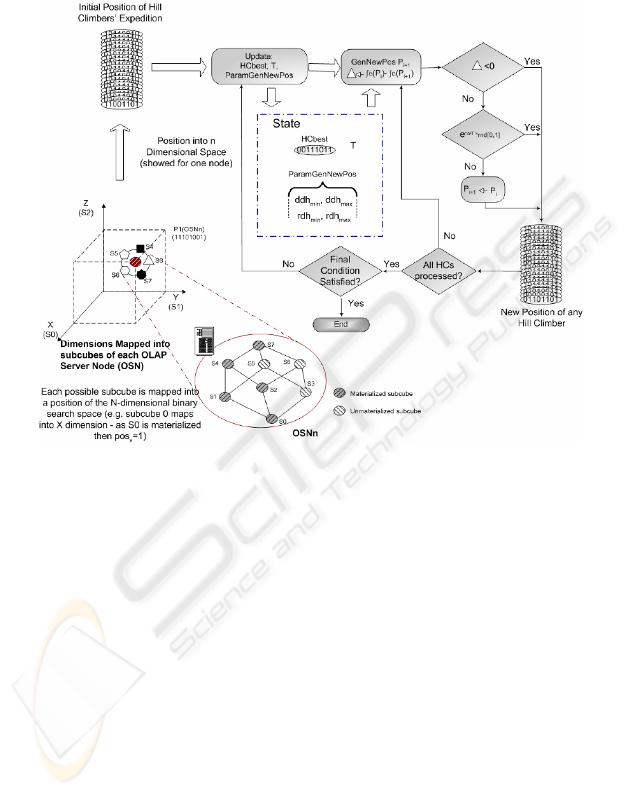
Figure 1: Functional scheme of HC-SA M-OLAP algorithm.

The process of rematerialization is made in an

identical way. The algorithm selects randomly a

dimension where the HC is at a 0 position and

changes its position to 1. In practice, the

corresponding subcube is materialized. All

parameters concerning this issue are user specified,

allowing the tuning of the algorithm.

Concerning to the fifth issue, the fitness function

(fa) of Figure 1, referring to definition 1, the

objective function is the minimizing of Cq(Q,

M)+Cm(M). We used the algorithms Multipipelining

Parallel Query Cost Calculation Algorithm with

Node Allocation by Constrained Reordering (PQA)

(Loureiro & Belo, 2006b) and Two Phase

Hierarchical Sequence with Multipipelining Parallel

Processing (2PHSMPP) (Loureiro & Belo, 2006b)

for estimating query and maintenance costs,

respectively.

Finally, for

and the cooling mechanism, we

decided for its setting by the user, implying a

preliminary tuning, having adopted a type 1 cooling

mechanism (as referred in section 2).

4 HC-SA M-OLAP ALGORITHM

Algorithm 2 presents the formal definition of the

proposed algorithm. As we can see, it uses the

solutions for the issues described in the last section.

The algorithm is divided into four main sections:

1. the initialization of parameters and objects, e.g.

the expedition of HCs;

2. the generation of the initial position of each HC,

its repairing to obey to the space constraint, the

computing of its fitness and the display of the

state;

3. the iterative module, where the moves of the HCs

are performed, as well as the evaluation of its

fitness, the updating of move’s control

parameters and the display of the state;

4. the returning of the best solution achieved.

Given the comments included, the algorithm

auto-explainable, and then we choose not to add any

further discussion. Among all rules, we highlighted

the one which accepts or rejects the movement of the

HC and the one which implements the movement.

ICSOFT 2007 - International Conference on Software and Data Technologies

Algorithm 2. HC-SA M-OLAP algorithm.

As we apply a per node space constraint, the hill

climbers’ moves may produce invalid solutions, as

when the materializing space is higher than the

maximal allowed space. In this work, we employ a

repair method, with the reposition of the HC by

randomly turning 1 positions to 0 until the HC’s

proposal is valid.

Input: L // Lattice (all granularity’s combinations and subcubes’ dependencies)

S=(S

... S

.) ; Q=(Q

... Q

) // Max. storage nodes’ space, query set (freq., dist.)

Pb // Base Parameters: Tf (type of Hc fixing), nOSN (number of OSNs),

MaximalSizeMaintWindow

Psa // Parameters of simulated annealing algorithm (NumHC, NumIter,

DefMovim, T

, α, tpGerac)

Mt // maintenance costs’ dependencies

P=(P

... P

.); X=(X

... X

.) // Nodes’ processing power; connections’ param.

Output: M // Materialized subcubes selected and allocated

Begin

1. Initialization:

M← { c

} // initialize with all empty nodes; node 0 has the base virtual relation

E← { }; d← NSCubes * nOSN // HC’ expedit. empty; d=dim. of search space

2. Generation, repairing, evaluation and showing the state of the initial HC’

expedit.

Repeat NumHC Times: // NumHC is the number of HCs of the expedition

While (MaintCost(hc))>MaximalSizeMaintWindow Do: // while position of

// generated hill climber (HC) doesn’t satisfy the maintenance constraint

hc ← GenerateHC(d) // generates the HC into a random position in d

For Each n Into MOLAP, Do: // for each OSN in MOLAP architecture

If (size(pos(hc),n)) >S

Then // if size of materialized subcubes proposed

// by solution of HC for node n > available mat. space in node n (S

)

Reposition(hc); // relocate HC into the dimensions mapped to node n

// to observe the space constraint

Next n

End While

E ←E

∪

hc; // add the hill climber to the expedition

fitness(hc)= f (hc, Q, M, X);

If fitness(hc)>hcBest Then hcBest ←fitness(hc); // updates hcBest (not really

// necessary, but interesting to show the initial best position)

End Repeat

ShowState(E); // shows the instant state of all hill climbers and hcBest

3. Expedition’s movement, fitness evaluation of each solution and state show:

Iter ←0; // iterations counter

While (Itr < NumIter) Do: // final condition is the number of iterations

T ← update (T); // T varies from T

until T→ 0 at each fuT iterations;

If iter>frozenI OR T<frozenT Then frozen ← true; // after frozenI

// iterations or when T is lower than a given value, the system is frozen

interv_Max_Unmat ←update(interv_Max_UnMat); // updates maximal

// number of bits which represent the position of each HC that was allowed

// to change from 1 to 0 in each iteration

intervMaxRemat ←update(intervMaxRemat) ; // updates maximal number of

// bits which represent the position of each HC that was allowed to change

// from 0 to 1 in each iteration

wU←rnd(interv_Max_UnMat); // generates the number of bits

// to change from 1 to 0 (un-materialize)

wR←rnd(interv_Max_ReMat); // generates the number of bits

// to change from 0 to 1 (materialize corresponding subcubes)

// Moves each HC according to the defined movement scheme

For Each hc Into E, Do:

While (MaintCost(hc))>MaximalSizeMaintWindow Do: // while new

// position of HC doesn’t verify the maintenance cost constraint

Repeat wU Times: // un-materilize wU sbcubes (changing bits - 1 to 0)

d ← select (D); // randomly selects node and subcube to un-materialize

hc(d) ← 0; // turns the bit (which represents the HC’s position) - 1 to 0

End Repeat

Repeat wR Times: // rematerilize wR sbcubes (changing bits - 0 to 1)

d ← select (D);// selects node and subcube to un-materialize with a

// prob. proportional to the available space into each node or to the

// relation available space x total space of each node; the subcube to

// rematerialize cannot imply the break of imposed space constraint

hc(d) ← 1; // turns the bit (which represents the HC’s pos. from 0 to 1)

End Repeat

End While

// Accepting or rejecting HC’s movement

delta ← f (hc (iter-1), Q, M, X) – f (hc (iter), Q, M, X); // computes the

// delta (loss of quality) concerning to HC movement,

// f is the fitness function

If delta > 0 AND frozen=true OR delta > 0 AND rnd([0,1))>e

-Δ/T

Then

hc(iter) ← hc(iter-1); // restore prev. pos. of the HC, reject. the new pos.

fitness(hc)= f (hc, Q, M, X);

If fitness(hc)>hcBest Then hcBest ←fitness(hc); // updates hcBest

Next hc;

ShowState(E); // shows the instant state of all hill climbers and hcBest

iter ← iter ++; // increments iterations’ counter

End While

4. Returning of result:

Return M(hcBest) // ret. M corresp. to the best posit. ever achieved by any HC

End

5 EXPERIMENTAL

PERFORMANCE STUDY

To perform the experimental study of the algorithms

we used the test set of Benchmark’s TPC-R (TPC-

R), selecting the smallest database (1 GB), from

which we used 3 dimensions (customer, product and

supplier). To broaden the variety of subcubes, we

added additional attributes to each dimension,

generating hierarchies, as follows: customer (c-n-r-

all); product (p-t-all) and (p-s-all); supplier (s-n-r-

all). Whenever the virtual subcube (base relation) is

scanned, this has a cost three times the subcube of

lower granularity.

We have used a 3 and 6 nodes’ M-OLAP

architecture (plus the base node), several randomly

generated query sets (of different sizes), and we

considered incremental maintenance costs. With this

environment we intend to evaluate the impact of the

following parameters onto the algorithm’s

performance: 1) the number of iterations, 2) the

value of T, 3) the number of HCs, 4) the number of

queries, and 5) the scalability of the algorithm

relating to the number of M-OLAP architecture’s

nodes. Given the stochastic nature of the algorithms,

all presented values are the average of 10 runs.

5.1 Parameters Tuning

Several preliminary tests were performed to tune

some parameters, whose selected values are shown

in Table 1. Other parameters, as fudri, the frequency

of T updating, and the iteration of the freezing of the

simulated annealing (when the simulated annealing

mechanism stops acting, thus the algorithm starts

behaving like a local search algorithm), are changed

accordingly to the selected values, for the associated

parameters. To make things clear, in this table, all

parameters are described.

As said above, the balance of the relation

exploration versus exploitation is changed along the

search process, by decreasing dsc and rsc range (at

each fudri – update frequency of dematerialization

and rematerialization interval). Reducing the range

of each HC’s journey with the running of the

algorithm implies that, in the beginning, the

exploration is favored; in opposite, in the later

OPTIMIZATION OF DISTRIBUTED OLAP CUBES WITH AN ADAPTIVE SIMULATED ANNEALING

ALGORITHM

phases, the same is valid for the exploitation (as the

range of the search is lower).

Table 1: Specified values for several parameters of HC-SA

M-OLAP algorithm.

Parameter Description Value

ddh

min

minimal number of

subcubes to dematerialize

ddh

max

maximal number of

subcubes to dematerialize

rdh

min

minimal number of

subcubes to rematerialize

rdh

max

maximal number of

subcubes to rematerialize

DecrD

the decrease of

ddh

min

and

ddh

max

DecrR

the decrease of r

min

and

max

InitPosGen

the way of generating the

initial position of each hill

climber

Random

5.2 Performed Tests

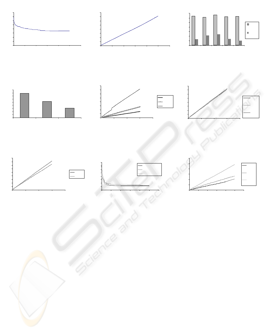
The first test tries to evaluate the impact of the

number of iterations over the quality of the achieved

solutions and also on the run-time of the algorithm.

We used 20 HCs and T

=30. Figure 2-a shows the

evolution of the quality of the solutions proposed by

the algorithm. As we can see, the quality of the

solutions has an initial fast improvement till about

100 iterations, followed by a slower evolution and

an almost null improvement beyond 300 iterations.

Moreover, another test, where 1000 iterations were

allowed, revealed a small improvement of the

quality of the solutions (3435 sec. for 500 iterations

versus 3411 sec. for 1000 iterations). Moreover, as

there is a linear relation between the number of

iterations and the run-time execution (as we can see

in Figure 2-b), the increase of the run-time doesn’t

pay off.

With the second test we tried to evaluate the

impact of the initial T

value over the quality of the

solutions. We used a limit of 300 iterations

(according to the conclusions of the last test). The

results are shown in Figure 2-c. As we can see, we

may say that the algorithm’s performance is almost

independent of T

(a difference of 1.2% on average

fitness and 4% for final fitness). Also, the plots don’t

allow deducing a behavior pattern, as they exhibit a

non monotonic variation. Watching the plots and

inspecting the relative values for the final solution’s

quality and its average, the value T

=30 seems to be

the one that ensures a better trade-off. Then, we

adopted this value for the remaining tests.

Another characteristic that is important to

evaluate, concerning to the algorithm’s behavior, is

the impact of the HCs’ number on the quality of the

achieved solutions and on the run-time. The plots of

Figure 2-d and 2-e show the obtained results. As we

can see, the plot of Figure 2-d shows that the number

of HCs has a reduced impact on the quality of the

achieved solutions (only 2.7 %). This is something

that was expected, given the absence of any

competition or cooperation mechanisms. E.g.

genetic algorithms are based on struggle for survival

and genoma diversity is a condition for evolution.

Also the learning process – through Pbest and Gbest

– which rules the particles’ dynamics in particles

swarm algorithm optimization, or stigmergy, in ants

algorithms, need a population of solutions. Here,

each HC acts independently of any other and there

isn’t any learning process. On the other side,

analyzing the plot of Figure 2-e, it is easy to

understand that there is an almost linear increase of

run-time with the HCs’ number. These two

evidences allowed us to conclude that it is

interesting to keep a low number of HCs, which

induces good solutions in a substantially inferior

time.

Finally, it is mandatory, as scalability is at

premium (recall the algorithm’s use to the M-OLAP

architecture), to evaluate the impact of the number

of queries and especially the nodes’ number (as we

are using the algorithm for optimizing an M-OLAP

system) on the run-time of the algorithm.

This way, for the first case, we used sets with 30,

60 and 90 queries, randomly generated. The run-

times are shown in plot of Figure 2-f. Observing this

plot, we may see that there is an almost null

dependency of the run-time in face of the number of

queries (the three lines are almost superposed). Also

observing Figure 2-g, we may see that an increase of

3 to 6 nodes in the M-OLAP architecture’s has

motivated a reduced increase of the run-time: for the

300 iterations there was only an increase of 10.6%.

These two observations show that the HC-SA M-

OLAP algorithm evidences a very good scalability,

being capable to deal with many queries and also

with M-OLAP architectures with many nodes.

Adding the easy scalability of hill climbing with the

simulated annealing, algorithm concerning to the

cube’s dimensionality (Kalnis et al. 2002), we have

an algorithm capable to scale in all directions.

ICSOFT 2007 - International Conference on Software and Data Technologies

Fitness Evolution

1000

2000

3000

4000

5000

6000

7000

8000

0 100 200 300 400 500 600

Iteration

Cost (s)

Run-Time

200

400

600

800

1000

1200

1400

1600

0 100 200 300 400 500 600

Iteration

Time (s)

Average and Final Fitness for Several T

Values

3400

3500

3600

3700

3800

3900

4000

4100

510203050

value

Cost (s)

Average

Fitness

Final

Fitness

(a) (b) (c)

Hill Climbers' Number Impact on the Quality of

the Achieved Solutions

3380

3400

3420

3440

3460

3480

3500

3520

3540

3560

20 40 100

Hill Climbers' Number

Cost

Hill Climbers' Number Impact on the Run-Time

500

1000

1500

2000

2500

3000

3500

4000

0 100 200 300 400

Iteration

Run-Time (s)

20 HCs

40 HCs

100 HCs

Queries' Number Impact on the Run-Time

100

200

300

400

500

600

700

800

0 100 200 300 400

Iteration

Run-Time (s)

Querie

(d) (e) (f)

Nodes' Number Impact on the Run-Time

100

200

300

400

500

600

700

800

900

0 100 200 300 400

Iteration

Run-Time (s)

3 OS Ns

6 OS Ns

HC-SA M-OLAP x Di-PSO M-OLAP x Ga M-OLAP

Algorithms Solution's Quality

4000

5000

6000

7000

8000

9000

10000

11000

12000

0 100 200 300 400 500 600

Iteration

Costs

HC-SA M-OLAP

Di-PSO M-OLAP

GA-P M-OLAP

Algorithms' Run-Time

1000

2000

3000

4000

5000

6000

0 100 200 300 400 500 600

Iteration

Run-Time (s)

HC-SA

M-OLAP

Di-PSO

M-OLAP

GA-P M

OLAP

(g) (h) (i)

Figure 2: Plots that show the results of the performed tests.

6 CONCLUSIONS AND FUTURE

WORK

This work proposes an adaptive simulated annealing

algorithm to optimize the selection and allocation of

a distributed cube for multi-node OLAP systems.

This algorithm improves existent proposals in three

distinct ways: 1) it uses a non-linear cost model to

support the estimation of the fitness of each solution,

simulating a parallel execution of tasks (using the

inherent parallelism of the M-OLAP architecture)

which deals with real world parameter values,

concerning to nodes, communication networks and

the measure value – time (Loureiro & Belo, 2006b);

2) it includes the maintenance cost into the cost

equation to minimize; 3) it also introduces simulated

annealing meta-heuristic onto the distributed OLAP

cube selection problem, extending the work of

(Kalnis et al. 2002) into the distributed arena. Also

concerning to this work, the HC-SA M-OLAP

algorithm includes a mechanism which dynamically

reduces the range of searched space in each iteration.

The run-time execution results show an easy

scalability of HC-SA M-OLAP in both directions:

the cube’s complexity and the number of nodes,

allowing to manage a distributed OLAP system,

capitalizing the advantages of computing and data

distribution, with light administration costs.

Also, observing the results of figure 3-h, the HC-

SA M-OLAP algorithm is competitive face to

standard genetic and particle swarm optimization

algorithms for this kind of problem. Moreover,

figure 3-i shows that the absolute run-time was also

the shortest of the three tested algorithms.

OPTIMIZATION OF DISTRIBUTED OLAP CUBES WITH AN ADAPTIVE SIMULATED ANNEALING

ALGORITHM

In the near future we intend to include this

algorithm into a general framework which includes

also a genetic, a co-evolutionary and a discrete

particle swarm algorithms. Any of these algorithms

may be used in its individuality or combined, where

each search agent may assume one of several forms

(a particle, an individual or a hill climber), switching

through a metamorphosis process. This mechanism

is also life inspired, as, in nature, the individuals of

many species assume different shapes in their

phenotype in different life epochs or under different

environmental conditions. Between each phenotypic

appearance many transformations occur, during the

so called metamorphosis, which many times

generates a totally different living being. Assuming

completely different shapes seems to be a way for

the living being to have a better global adaptation,

changing its ways to a particular sub-purpose. E.g.

for the butterflies, the larva state seems to be ideal

for feeding and growing; the butterfly seems to be

perfectly adapted to offspring generating, especially

increasing the probability of diverse mating and

colonization of completely new environments (recall

the spatial range that a worm could run and the

space that a butterfly could reach and search). But

all these states contribute to the main purpose:

struggle for survival.

While designing this algorithm and keeping in

mind some knowledge about each meta-heuristics’

virtues and limitations that are somewhat disjoint,

we figured that, if combined, they may generate a

globally better algorithm. What is more, this schema

could be easily implemented as a unified algorithm

because of the similarities between the solutions’

evaluation scheme and the easy transposing of

solutions’ mapping. This new meta-heuristic may be

denoted as “metamorphosis algorithm”, which is

expected to have an auto-adaptation mechanism.

ACKNOWLEDGEMENTS

The work of Jorge Loureiro was supported by a

grant from PRODEP III, acção 5.3 – Formação

Avançada no Ensino Superior, Concurso N.º

02/PRODEP/2003.

REFERENCES

Bauer, A., and Lehner, W., 2003. On Solving the View

Selection Problem in Distributed Data Warehouse

Architectures. In Proceedings of the 15th International

Conference on Scientific and Statistical Database

Management (SSDBM’03), IEEE, pp. 43-51.

Gupta, H. and Mumick, I.S., 1999. Selection of Views to

Materialize under a Maintenance-Time Constraint. In

Proc. of the International Conference on Database

Theory.

Harinarayan, V., A. Rajaraman, and J. Ullman, 1996.

Implementing Data Cubes Efficiently. In Proceedings

of ACM SIGMOD, Montreal, Canada, pp. 205-216.

Kalnis, P., Mamoulis, N., and D. Papadias, 2002. View

Selection Using Randomized Search. In Data

Knowledge Engineering, vol. 42, number 1, pp. 89-

111.

Kirkpatrick, S, Gelatt, C. D. and Vecchi, M. P., 1983.

Optimization by Simulated Annealing. Science, vol.

220, pp. 671-680, 1983.

Liang, W., Wang, H., and Orlowska, M.E., 2001.

Materialized View Selection under the Maintenance

Cost Constraint. In Data and Knowledge Engineering,

37(2) (2001), pp. 203-216.

Lin, W.-Y., and Kuo, I.-C., 2004. A Genetic Selection

Algorithm for OLAP Data Cubes. In Knowledge and

Information Systems, Volume 6, Number 1, Springer-

Verlag London Ltd., pp. 83-102.

Loureiro, J., and Belo, O., 2006a. Evaluating Maintenance

Cost Computing Algorithms for Multi-Node OLAP

Systems. In Proceedings of the XI Conference on

Software Engineering and Databases, Sitges,

Barcelona, October 3-6, 2006.

Loureiro, J., and Belo, O., 2006b. Establishing more

Suitable Distributed Plans for MultiNode-OLAP

Systems. In Proceedings of the 2006 IEEE

International Conference on Systems, Man, and

Cybernetics, Taipei, Taiwan, October 8-11, pp. 3573-

3578.

Loureiro, J. and Belo, O, 2006c. An Evolutionary

Approach to the Selection and Allocation of

Distributed Cubes. In Proceedings of the 2006

International Database Engineering & Applications

Symposium (IDEAS2006), Delhi, India, December 11-

14, 2006.

Loureiro, J. and Belo, O., 2006d. Swarm Intelligence in

Cube Selection and Allocation for Multi-Node OLAP

Systems. To appear in Proceedings of the 2006

International Conference on Systems, Computing

Sciences and Software Engineering (SCSS 06).

Transaction Processing Performance Council (TPC): TPC

Benchmark R (decision support) Standard

Specification Revision 2.1.0. tpcr_2.1.0.pdf, available

http://www.tpc.org.

Zhang, C., Yao, X., and Yang, J., 2001. An Evolutionary

Approach to Materialized Views Selection in a Data

Warehouse Environment. In IEEE Trans. on Systems,

Man and Cybernetics, Part C, Vol. 31, n. 3.

ICSOFT 2007 - International Conference on Software and Data Technologies