
A CASE STUDY ON THE APPLICABILITY OF SOFTWARE
RELIABILITY MODELS TO A TELECOMMUNICATION
SOFTWARE
Hassan Artail, Fuad Mrad and Mohamad Mortada
Electrical and Computer Engineering, American University of Beirut, Beirut, Lebanon
Keywords: System testing, quality assurance, system reliability, software failures, CASRE (Computer Aided Software
Reliability Estimation), Software Reliability, inter-failure times, Time-Between-Failures.
Abstract: Faults can be inserted into the software during d
evelopment or maintenance, and some of these faults may
persist even after integration testing. Our concern is about quality assurance that evaluates the reliability and
availability of the software system through analysis of failure data. These efforts involve estimation and
prediction of next time to failure, mean time between failures, and other reliability-related parameters. The
aim of this paper is to empirically apply a variety of software reliability growth models (SRGM) found in
the CASRE (Computer Aided Software Reliability Estimation) tool onto real field failure data taken after
the deployment of a popular billing software used in the telecom industry. The obtained results are assessed
and conclusions are made concerning the applicability of the different models to modeling faults
encountered in such environments after the software has been deployed.
1 INTRODUCTION
Test procedures should be thorough enough to
exercise system functions to everyone's satisfaction:
user, customer, and developer. There are several
steps involved in testing a software system. They
comprise unit testing, integration testing, acceptance
testing, and installation testing. If the tests are
incomplete, faults of various types may remain
undetected, while on the other hand, complete and
early testing can help not only to detect faults
quickly, but also to isolate causes more easily
(Pfleeger, 2001).
This paper presents a case study, in which
so
ftware failures were analyzed after the completion
of the software development and testing phases
before deployment at the customer premises. This
study is different from the traditional software
reliability analysis in the sense that most reported
cases were based on the development and testing
phases or the operational phase, but seldom
considered the software installation and
implementation phases at the client site. Another
important aspect that is taken up in this work is the
examination of the applicability of known software
reliability models to the considered system, given
that such models were primarily developed to handle
reliability analysis during the software testing phase
(typically at the vendor’s site) while assuming fast
error removal.
The studied product is a multi-component billing
soft
ware used by a reputable GSM operator. It
interacts with an Oracle database and with Siemens’
HLR telecommunication systems, and includes
components that use the client/server model to serve
more than 1300 users who access the server from
their Java based client interfaces. It is worth noting
that the vendor’s support team has prior experience
with the implementation of such products in similar
environments, but never with the same combination
of client profile and third party products.
The presented research is based on collected
real life
failure data for a component of the software.
A comparative analysis of the failure data using
various statistical tests was executed in order to
show the statistical model that best-fits this
particular situation. A projection was then made
regarding the underlying component reliability, or in
other words, the maximum allowable execution time
before failing again for a particular fault.
178
Artail H., Mrad F. and Mortada M. (2007).
A CASE STUDY ON THE APPLICABILITY OF SOFTWARE RELIABILITY MODELS TO A TELECOMMUNICATION SOFTWARE.
In Proceedings of the Second International Conference on Software and Data Technologies - SE, pages 178-183
DOI: 10.5220/0001347401780183
Copyright
c
SciTePress

2 PREVIOUS WORK
Since the characteristics of a software system cannot
always be measured directly before delivery, indirect
measures can be used to estimate the system’s likely
characteristics. Several software reliability (SR)
models with basic SR parameters were developed. In
contrast to most reliability models that assume
instantaneous fault removal, Jeske, Zhang, and Pham
(2001) and then Zhang, Teng, and Pham (2003)
stressed that a fault may be encountered more than
once before it is ultimately removed and that new
faults may be introduced to the software due to
imperfect debugging. Mullen (1998) argued that
there is a time lag which most conventional software
reliability models ignore. They considered the fault
removal process with different scenarios using the
state space view of the Non-Homogeneous Poisson
Process (NHPP). Teng and Pham (2002) considered
the error introduction rate and error removal
efficiency as the key measures for reliability growth
across multiple versions of a software system that
was subject to continuous fault removal. The
classical reliability theory was extended in the work
of Goseva-Popstojanova and Trivedi (2000) to
consider a sequence of possibly-dependent software
runs versus failure correlation. A model, suggested
by Singpurwalla (1998), involved concatenating the
failure rate function while assuming that the time to
next failure was greater than the average of past
inter-failure times. Fault removal, repair time, and
remaining number of faults were handled using a
non-homogeneous continuous time Markov chain.
A criterion was proposed by Nikora and Lyu
(1995) for selecting the most appropriate software
reliability model from six models: Jelinski-Moranda,
Geometric, Littlewood-Verral, Musa Basic, Musa-
Okumoto, and NHPP. The goodness-of-fit test based
on the Kolmogorov-Smirnov distance was not
sensitive enough to choose the best model, but it was
used as a preliminary step for filtering unsuitable
ones. Huang, Kuo, Lyu, and Lo (2000) verified that
existing reliability growth models can be derived
based on a unified theory of well-known means:
weighted arithmetic, geometric, and harmonic.
According to Gokhale, Marinos, Lyu, and Trivedi
(1997), commercial software organizations focus on
the residual number of faults as a measure of
software quality. A model was proposed to address
the number of residual defects during the operational
phase. Minyan, Yunfeng, and Min (2000) stressed
that neither practitioners nor experts could choose a
model beforehand since the assumptions of each
model were difficult to prove.
3 CASE STUDY AND APPLIED
RELIABILITY ANALYSIS
Software reliability models can be largely
categorized into two sets: static models where
attributes of the software module are utilized to
estimate the number of defects in the software, and
dynamic models which utilize parametric
distributions and defect patterns to evaluate the end
product reliability. Musa and Okumoto classified
dynamic models in terms of five attributes (Musa,
2004): 1) time, 2) category (number of failures), 3)
type (distribution of the number of failures), 4) class
(functional form of failure intensity in terms of
time), and 5) family (functional form of failure
intensity in terms of expected number of failures).
3.1 Considered Models
The reliability models discussed in this paper are
based on the time domain using either the elapsed
time between failures or the number of failures over
a given period of time. Musa (2004) identified two
sets of reliability models in accordance with time
between failure (TBF) and fault count models. The
first group includes the Jelinski-Moranda, Non-
Homogeneous Poisson Process (NHPP), Geometric,
Littlewood-Verral Quadratic, Littlewood-Verral
Logarithmic, Musa Basic, and Musa Logarithmic.
The second group comprises the Yamada S-Shaped,
NHPP, Schneidewind, Generalized Poisson, and
Brook and Motley’s models.
3.2 System Description
The field failure data are taken from error log files
that date back to the month of February 2006, during
the initial software implementation and integration
of the BSCS version 7 billing software on a
clustered Tru64 Unix platform with an Oracle 9i
RAC database system. The components of the BSCS
billing software are integrated with other third party
interfaces like the HLR system of Siemens and the
Oracle production databases, which include detailed
information and billing data of GSM subscribers.
The connection with Siemens HLR is crucial since it
involves activation of many GSM subscriber
services. The interface with the Oracle database is
equally critical due to the fact that all data are kept
inside various production and rating databases.
Furthermore, these data are accessed from around
1300 concurrent users using either an SQL interface
or Java client programs through a LAN or a WAN.
A CASE STUDY ON THE APPLICABILITY OF SOFTWARE RELIABILITY MODELS TO A
TELECOMMUNICATION SOFTWARE
179
The failure data was examined for any
inherent trend for applicability of software reliability
growth models. This is an important step where the
data content implies either a growth for time-
between-failures or decrease of failure counts as
time progresses. Two data trend tests were used:
running average test and Laplace test. The former
computes the running average of time between
successive failures or count of failures per time
interval. For time between failures, if the running
average increases with failure number, a reliability
growth is implied, while for failure count data, if the
running average decreases with time then reliability
growth is indicated. On the other hand, the Laplace
test computation is based on the null hypothesis that
occurrences of failures can be described as a
homogeneous Poisson process. If the test metric
decreases with increasing failure number, the null
hypothesis is rejected in favor of reliability growth
at an appropriate significance level. Otherwise, the
null hypothesis is rejected in favor of decreasing
reliability (Nikora, 2000).
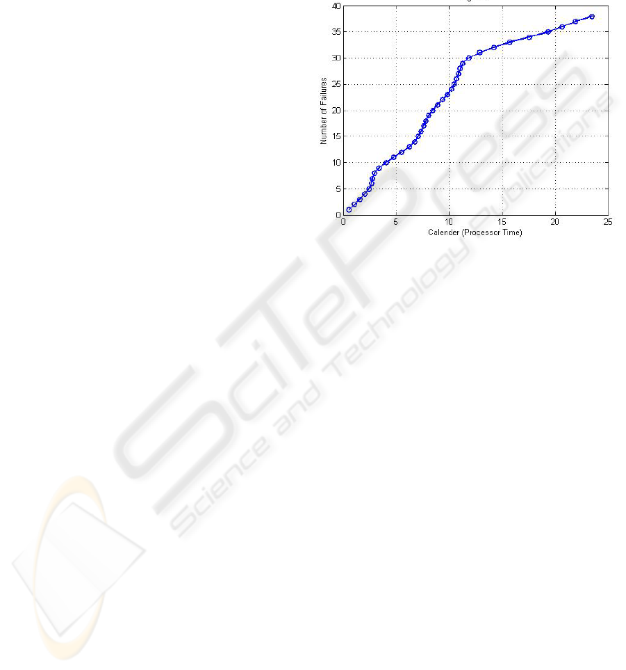
3.3 Raw Reliability Data Analysis
The cumulative number of 39 failures against their
respective execution times is shown in Figure 1,
where a saturation-like curve behavior is observed.
In the subsequent sections, we divide our execution
time failure data into two sets: time-between-failure
and failure-count sets. This allows for applying a
different set of models for every data type and
having a better view of the reliability of the software
under study. Moreover, our analysis for every data
type- reliability model combination is done using
two estimation methods: maximum likelihood
estimation (MLE) and least squares estimate (LSE).
The choice of the best software reliability model
that mostly fits a particular set of data type, time-
between-failures, or failures count is done using the
following steps (Nikora and Lyu, 1995):
1. Apply a goodness of fit test to determine which
model fits the input data for a specified
significance level.
2. If more than one set of results are a good fit:
a. Choose the most appropriate model(s)
based on the prequential likelihood.
b. In case of a tie, use the model bias trend.
3. If no models provide a good fit to the data:
a. Choose the most appropriate model(s)
based on the prequential likelihood.
b. Use techniques, such as forming linear
combinations of model results or model
recalibration to increase accuracy.
c. Apply the goodness of fit test to the
adjusted model results and identify those
that are a good fit to the data.
4. Finally, the models are ranked using the
CASRE tool according to the following when
applicable: prequential likelihood, Model bias,
Bias trend, Model noise, and Goodness-of-fit.
Figure 1: Cumulative number of failures of PIH
component against processor execution time (hours).
3.4 Time-Between-Failures (TBF)
Figure 2 shows the actual time-between-failure data,
filtered with a Hann window. A running arithmetic
average test showed a reliability growth starting at
failure point 27 and onwards. The Laplace test
showed the software starting to exhibit reliability
growth at the 5% significance level until about the
34th failure, at which point the Laplace test statistic
assumes a value less than -1.64495. The inserted
failure data set into the CASRE software tool
consisted of 38 data points. For the purpose of this
test, the CASRE tool was set with a data range from
27 to 35 time-between-failures data points with the
models parameters estimation end point at 30, i.e.
training the models parameters from data range 27-
30 before fixing them. The number of steps past the
last data point in the modelling range, for which
predictions are made, is selected to be 4. This way,
one could see how close are each model’s first 3
failure data predictions to the true ones and look into
the next future failure time and reliability.
ICSOFT 2007 - International Conference on Software and Data Technologies
180
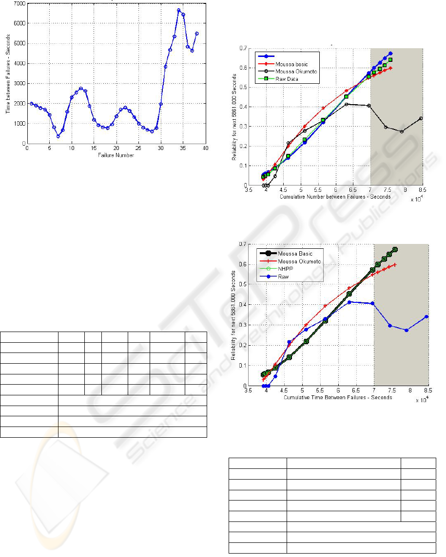
Figure 2: Filtered raw data plot for TBF.
3.4.1 TBF Analysis with the MLE Method
Table 1 is obtained after running the CASRE
software tool with the selected models. The
goodness of fit test is done first to determine which
models are fit to the data. We consider the first three
ranked reliability models and displayed their various
estimates and predicted outputs. The top three fitting
models in this case were: Musa-Okumoto, ULC, and
Musa basic. They are ranked according to their
Kolmogorov-Smirnov (KS) distance test value.
Table 1: Model goodness of fit for TBF using MLE.
Model -In PL Bias Trend Noise Distance Rank
Musa-Okumoto 39.28 0.52 0.34 1.27 0.42 1
ULC 39.51 0.48 0.36 1.13 0.38 2
Musa Basic 40.03 0.46 0.34 1.39 0.29 3
NHPP (TBE) 40.03 0.46 0.34 1.39 0.29 4
MLC 40.03 0.46 0.39 0.07 0.29 5
DLC/S/4 Did not fit data at given significance level
ELC Did not fit data at given significance level
Geometric Did not fit data at given significance level
Quadratic LV Did not fit data at given significance level
Figure 3 shows the fits of three top-ranked reliability
models onto the actual TBF data, where the models’
estimates are plotted in the shaded region.
3.4.2 TBF Analysis with LSE Method
The information in Table 2 is obtained after running
the CASRE software tool with the selected models.
Out of the models that pass the fit test, we consider
the Musa Basic, NHPP, and Musa-Okumoto models.
As implied in the data in Table 2, the bias,
prequential likelihood, and relative accuracy are not
computed when employing the least squares
estimation method. Figure 4 presents the fit of the
three models onto the actual data points. Similar to
the MLE case, the estimates of the software
reliability models are plotted in the shaded region.
Figure 3: Models' estimated and predicted reliability for
TBF using MLE.
Figure 4: Models estimated and predicted reliability for
TBF using LSE.
Table 2: Model goodness of fit for TBF using LSE.
Model Distance Rank
Musa Basic 0.29 1
NHPP (TBE) 0.29 2
MLC 0.29 3
ULC 0.38 4
Musa-Okumoto 0.42 5
ELC Did not fit data at given significance level
Quadratic LV Did not fit data at given significance level
Geometric Did not fit data at given significance level
3.5 Failure Counts (FC)
Figure 5 shows the Laplace test results illustrating
reliability growth at the 5% significance level until
A CASE STUDY ON THE APPLICABILITY OF SOFTWARE RELIABILITY MODELS TO A
TELECOMMUNICATION SOFTWARE
181
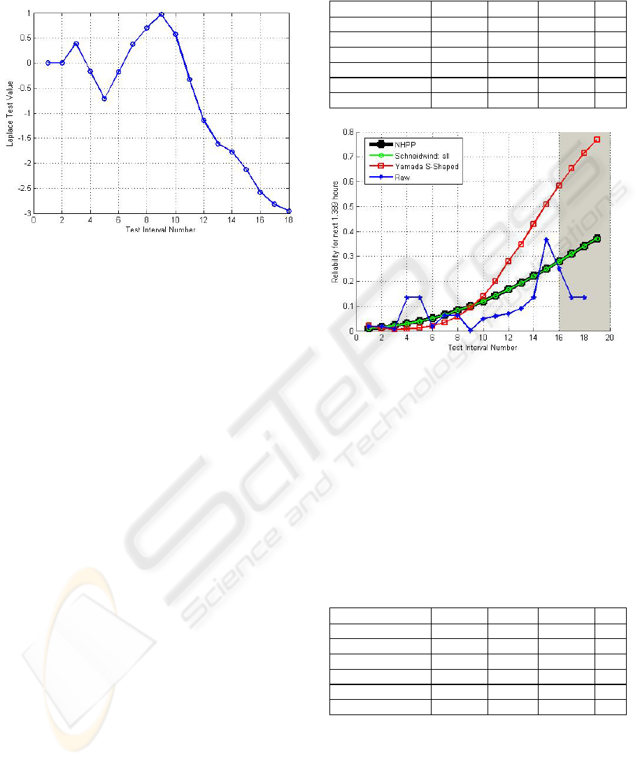
about the 13th failure, at which the Laplace test
assumes a value less than -1.64495.
Figure 5: Laplace trend test on raw data for FC
The failure count data set into the CASRE software
tool consists of 18 data points. For this test, the tool
was set up with a data range from 1 to 15 failure-
count data points, with the models parameters
estimation end point at 12. This implies that the
models’ parameters were trained from the first 12
data points before fixing them. The number of steps
past the last data point in the modelling range, for
which predictions are to be made, is selected to be 4.
We can see how each model’s first 3 failure data
predictions came close to the true ones and also look
into the next future failure count and reliability.
3.5.1 FC Analysis with MLE Method
Table 3 is obtained after running the CASRE
software tool with the selected software reliability
models specific to the failures count case, which
divides the x-axis into equal interval of time with a
length of 1.389 hours. The fit test is done first in
order to determine which models best fit the actual
real field failure data. We then considered the three
reliability models that passed the test, as shown in
the table. It is noted that the ranking was done in
accordance with the Chi-Square (χ
2
) value where by
smaller values led to a higher ranking.
As was done earlier, we illustrate the outcome
of the fit test against the raw data in Figure 6.
Table 3: Fit results for FC using MLE. χ
2
denotes Chi-
Square and the fourth column stands for significance level.
Model
χ
2
5% Fit? Sig. (%) Rank
Gen. Poisson 10.16 No 3.78 --
NHPP (intervals) 5.49 Yes 24.04 1
Schick-Wolverton 10.16 No 3.78 --
Schneid.-Cum. 1st 31.34 No 0.0 --
Schneidewind:all 5.49 Yes 24.04 2
Yamada S-Shaped 8.31 Yes 8.93 3
Figure 6: Estimated/predicted reliability for FC using
MLE.
3.5.2 FC Analysis with the LSE Method
Table 4 applies to the failure count case that divides
the x-axis into equal interval of time with a length of
1.389 hours per interval. The three top passing
models from the fit test are illustrated in the table:
Generalized Poisson, Schick-Wolverton, and
Schneidewind: all. The ranking was performed
according to the value of the Chi-Square test value,
with a smaller value leading to a higher ranking.
Table 4: Goodness of fit results for FC using LSE.
Model
χ
2
5% Fit? Sig. (%) Rank
Gen. Poisson 5.38 Yes 25.05 1
NHPP (intervals) 10.85 No 2.83 --
Schick-Wolverton 5.38 Yes 25.05 2
Schneid.-Cum. 1st 31.34 No 0.0 --
Schneidewind:all 5.93 Yes 24.04 3
Yamada S-Shaped 8.08 Yes 8.93 4
The fit of the three-ranked reliability models onto
the actual failure data is illustrated in Figure 7, and
where the models’ data point estimates are plotted in
the shaded region.
ICSOFT 2007 - International Conference on Software and Data Technologies
182
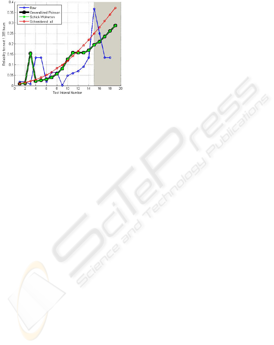
Figure 7: Estimated/predicted reliability for FC using LSE.
4 CONCLUSIONS
Although some reliability models fitted well the
time-between-failure data, all considered models
with both maximum likelihood (MLE) and least
squares (LSE) methods did not initially pass the
goodness-of-fit test when applied to the whole range
of the non-filtered data. Existing reliability models
considered fault removal upon detection and hence,
could not initially be suitable for our application
since the detected faults were never removed during
software installation and integration. The developers
actually worked around these faults to decrease their
frequency of occurrence, until it was time for the
next patch that dealt specifically with these faults.
Based on our findings, it is preferable to stick to
the software reliability growth models (SRGM)
dealing with failure counts and use the least square
estimation (LSE) method. The prequential likelihood
test can not be obtained when using the LSE
method, so instead, the Chi-Square test was
performed. The Generalized Poisson SRGM exhibits
a better fitness over all the other models, like the
Musa Okumoto, Musa Basic, and NHPP models. In
fact, when comparing the predictions of the four
reliability modules, we can see that the Generalized
Poisson predicted more faithfully the software
reliability than the other three models. For instance,
to achieve a 30% reliability of the software, the
implementation and integration phase should run for
around 15.27 hours in case of both Musa-Okumoto
and Musa Basic models, for around 22.5 hours in
case of Non-Homogeneous Poisson Process
(NHPP), and for around 26.39 hours in case of the
Generalized Poisson model. Moreover, the LSE
method performs much better when compared with
MLE in the short data range. Hence, the least square
estimation method adapts faster than the maximum
likelihood estimation method on a small range of
failure data points. However, on the long run, MLE
performs better than LSE if the failure data range
increases considerably.
REFERENCES
Gokhale, S., Marinos, P., Lyu, M., Trivedi, K., 1997.
Effect of Repair Policies on Software Reliability,
12th
Annual Conference on Computer Assurance, IEEE
Computer Society.
Goseva-Popstojanova, K., Trivedi, K., 2000. Failure
Correlation in Software Reliability Models. IEEE
Transactions on Reliability, 49(1),
pp. 37-48.
Huang, C., Kuo, S., Lyu, M., Lo, H., 2000. Quantitative
Software Reliability Modeling from Testing to
Operation. 11th International Symposium on Software
Reliability Engineering,
IEEE Computer Society.
Jeske, D., Zhang, X., Pham, L., 2001. Accounting for
Realities when Estimating the Field Failure Rate of
Software. 12th International Symposium on Software
Reliability Engineering,
IEEE Computer Society.
Minyan, L., Yunfeng, B., Min, C., 2000. A Practical
Software-Reliability Measurement Framework Based
on Failure Data. International Symposium on Product
Quality and Integrity,
IEEE Computer Society Press.
Mullen, R., 1998. The Lognormal Distribution of Software
Failure Rates: Application to Software Reliability
Growth Modeling. 9th International Symposium on
Software Reliability Engineering,
IEEE Computer
Society
.
Musa, J., 2004. Software Reliability Engineering: More
Reliable Software Faster and Cheaper. McGraw-Hill,
2
nd
edition.
Nikora, A., Lyu, M., 1995. An Experiment in Determining
Software Reliability Model Applicability, 6th
International Symposium on Software Reliability
Engineering
, IEEE Computer Society.
Nikora, A., 2000. Computer Aided Software Reliability
Estimation User’s Guide, available online at:
http://www.openchannelfoundation.org/projects/
CASRE_3.0
Pfleeger, S., 2001. Software Engineering. Prentice Hall.
Singpurwalla, N., 1998. Software Reliability Modeling by
Concatenating Failure Rates, 9th International
Symposium on Software Reliability Engineering, IEEE
Computer Society
.
Teng, X., Pham, H., 2003. A Software-Reliability Growth
Model for N-Version Programming Systems. IEEE
Transactions on Reliability, 51(3),
pp. 311-321.
Zhang, X., Teng, X., Pham, H., 2001. Considering Fault
Removal Efficiency in Software Reliability
Assessment. IEEE Transactions on Systems, Man, and
Cybernetics – Part A, 33(1),
pp. 114-120.
A CASE STUDY ON THE APPLICABILITY OF SOFTWARE RELIABILITY MODELS TO A
TELECOMMUNICATION SOFTWARE
183
