STABILIZATION OF UNCERTAIN NONLINEAR SYSTEMS VIA

PASSIVITY FEEDBACK EQUIVALENCE AND SLIDING MODE

Rafael Castro-Linares

CINVESTAV-IPN, Department of Electrical Engineering, Av. IPN 2508, Col. San Pedro Zacatenco, 07360 Mexico, D.F., Mexico

Alain Glumineau

IRCCyN, UMR 6597 CNRS, Ecole Centrale de Nantes, 1 rue de la Noe, 44321 Nantes Cedex 03, France

Keywords:

Passivity feedback equivalence, sliding mode technique, stabilization, uncertain nonlinear systems.

Abstract:

In this paper, a sliding mode controller based on passivity feedback equivalence is developed in order to

stabilize an uncertain nonlinear system. It is shown that if the nominal passive system obtained by feedback

equivalence is asymptotically stabilized by output feedback, then the uncertain system remains stable provided

the upper bounds of the uncertain terms are known. The results obtained are applied to the model of a magnetic

levitation system to show the controller methodology design.

1 INTRODUCTION

In the last decade the concept of passivity has been

mainly used in the stability analysis of continous-time

state-space nonlinear systems (Cai and Han, 2005;

Mahmoud and Zribi, 2002) and to analyze the sta-

bility properties of nonlinear interconnected systems

and special cascaded structures (Byrnes et al., 1991;

Ortega, 1991). Besides, an important question arises

when the model of the system contains uncertain el-

ements such as constant or varying parameters that

are not known or imperfectly known. Under such

imperfect knowledge of the model, the feedback that

makes the uncertain system passive is no longer ro-

bust. Some works using nonlinear adaptive control

have been recently devoted to this issue (Su and Xie,

1998; Duarte-Mermoud et al., 2002). On the other

hand, the control of nonlinear systems with uncertain-

ties via the sliding mode technique has been widely

studied in the literature to attain robust control struc-

tures; see, for example the results presented in (Tunay

and Kaynak, 1995).

The goal of the present paper is to develop a con-

troller via passivity feedback equivalence and sliding

modes that permits to stabilize an uncertain nonlin-

ear system. Stabilization is obtained whenever the

passive system associated to the nominal system is

asymptotically stabilized by output feedback; a sim-

ilar approach was presented in (Loria et al., 2001)

where a different sliding surface is proposed. The

study is completed by means of an example of height

distance regulation in the model of a magnetic levita-

tion system.

2 PASSIVITY EQUIVALENCE

AND STABILIZATION USING

SLIDING MODES

One considers uncertain MIMO nonlinear systems

described by



˙x = f(x) +∆f(x) + (g(x) + ∆g(x))u,

y = h(x)

(1)

where x ∈ ℜ

is the state vector, u ∈ ℜ

is the in-

put vector, y ∈ ℜ

is the output vector. f and the p

columns of the matrix g are C

∞

vector ﬁelds, and the

p components of the vector h are C

∞

functions. ∆f

and the p columns of the matrix ∆g are smooth vector

ﬁelds deﬁned on ℜ

which represent the model un-

certainties. In addition, we suppose, without loss of

generality and after a possible coordinates shift, that

f(0) = 0 and h(0) = 0. The MIMO nonlinear system

(1) without uncertainties, also referred as the nominal

system, is described by

Σ :



˙x = f(x) + g(x)u,

y = h(x).

(2)

339

Castro-Linares R. and Glumineau A. (2007).

STABILIZATION OF UNCERTAIN NONLINEAR SYSTEMS VIA PASSIVITY FEEDBACK EQUIVALENCE AND SLIDING MODE.

In Proceedings of the Fourth International Conference on Informatics in Control, Automation and Robotics, pages 339-342

DOI: 10.5220/0001614603390342

 SciTePress

This is, Σ is given by Σ

with ∆f(x) = 0 and ∆g(x) =

0 for all x.

Let us now assume that the nominal system Σ

has relative degrees r

= 1,...,r

= 1, that the ma-

trix L

h(0) is nonsingular and that it is weakly min-

imal phase; this is, system (2) is locally equiva-

lent to a passive system (Byrnes et al., 1991). Let

S(y, v) = col{S

(y,v),.. .,S

(y,v)} be an p dimen-

sional smooth function that we refer as the switching

function where v is a new input signal. In this work,

we set S(y, v) as

S(y, v) = y−

v(τ)dτ. (3)

In the sliding mode, S =

S = 0, and the state trajectory

of the nominal system is constrained to evolve on the

sliding surface M

by the so-called equivalent control

u = u

. If an initial point does not belong to M

, the

attractivity condition (

S ≤ −λ with λ > 0 must be

satisﬁed in a neighbourhood of M

, so that this sur-

face becomes attractive (Utkin, 1992). The control

law which permits to reach the sliding surface can be

obtained from the expression

S = −F(S) where F(S)

is, in general, a discontinuous vector function of its

arguments.

Writting the uncertain system (1) in the new co-

ordinates (y, z), with z being a set of complimentary

coordinates, and substituting the feedback

u = u

slid

= b(y, z)

−1

[−F(S) − a(y, z) + v]. (4)

where b(y, z) is nonsingular for all (y,z) near

(0,0) and setting F(S) = Γsign(S) where

sign(S) := col{sign(S

),. . .,sign(S

)} and

Γ > 0, one has











˙y = v− Γsign(S) + ∆a(y,z)

+∆b(y, z)b

−1

(y, z)(−a(y, z) − Γsign(S) + v)

˙z = f

∗

(z) + p(y,z)y+ {

∑

i=1

(y, z)y

+∆p(y,z)y+ {

∑

i=1

∆q

(y, z)y

∑

i=1

∆r

(y, z)y

}Γsign(S)

(5)

where p(y,z) and the q

(y,z)’s are suitable matrices

of appropriate dimensions and ˙z = f

∗

(z) are the so

called zero dynamics of the nominal system. ∆p(y,z),

the ∆q

(y,z)’s, and the ∆r

(y,z)’s are matrices which

represent the terms associated to the uncertainties in

the z variables. ∆a(y,z) and ∆b(y, z) represent the un-

certainties associated to the y variable.

Since it is assumed that the nominal system is

weakly minimal phase, its zero dynamics are Lya-

punov stable with a time-independent and C

Lya-

punov function W

∗

(z), and one chooses the signal v

as (Byrnes et al., 1991)

v = [I + M(y,z)]

−1

[−(L

p(y,z)

∗

(z))

+ w] (6)

where M(y,z) = [(L

∗

)

·· · (L

∗

)

]

. This

choice makes the closed-loop nominal system

[ ˙y

˙z

] =

f(y,z) + g(y,z)w passive from the input w

to the output y. Assuming that this passive system

is also locally zero state detectable

, its equilibrium

(y,z) = (0,0) can be can be made asymptotically sta-

ble by the simple output feedback w = −φ(y) with

φ(0) = 0 and y

φ(y) > 0 for each y 6= 0. Let us deﬁne

deﬁne ξ = (y,z) and substitute the assignment (6) to-

gether with w = −φ(y) into the uncertain system (5).

The resulting closed-loop system can then be written

ξ =

F(ξ) +

G(ξ) (7)

where

F(y,z) =

f(y,z)− ¯g(y,z)φ(y),

G(ξ) =

(ξ)+

(ξ)

and

(y,z) =



(y,z)



(y,z) =



(y,z)



(8)

with

(y, z) = −Γsign(S) + ∆a(y,z)

+∆b(y, z)b

−1

(y, z)(−a(y, z) − Γsign(S)

+[I + M(y, z)]

−1

[−(L

p(y,z)

∗

(z))

− φ(y)]),

(y, z) = ∆p(y, z)y+ {

∑

i=1

∆r

(y, z)y

}Γsign(S)

∑

i=1

∆q

(y, z)y

}[I

+M(y, z)]

−1

[−(L

p(y,z)

∗

(z))

− φ(y)].

We now assume that the uncertain terms satisfy the

uniform bounds

(ξ) k≤ δ

, k

(ξ) k≤ δ

(9)

for all ξ ∈ D where D = {ξ ∈ ℜ

:|| ξ ||< r} with r > 0

or, equivalently,

G(ξ) k≤ δ

+ δ

= δ (10)

for all D. Notice that ξ = 0 is a locally asymptoti-

cally equilibrium point of the system

ξ =

F(ξ) and

one can then assure, by using the Lyapunov approach,

that for all bounded initial conditions ξ(0), the solu-

tion ξ(t) of the uncertain system (7) is locally ulti-

mately bounded for t ≥ 0. Moreover, one can show

that the sliding surface M

becomes attractive for any

initial point ξ(0) ∈ D if

Γ ≥ [1− k ∆bb

−1

sign(S) k]

−1

[k ∆a k

+ k ∆bb

−1

([I + M]

−1

[−(L

∗

)

− φ] − a) k +λ]

(11)

whenever k ∆bb

−1

sign(S) k6= 1, with λ being a

nonzero positive constant (see, in particular, (Khalil,

1996), Lemma 5.3, Chapter 5, p. 216).

A system (2) is locally zero-state detectable if there

exists a neighbourhood U of 0 such that, for all x ∈ U,

y(t) = h(x(t)) ≡ 0 implies that x(t) → 0 as t → ∞. It is said

to be locally zero-state observable if there exists a neigh-

bourhood U of 0 such that, for all x ∈ U, y(t) = h(x(t)) ≡ 0

implies that x(t) = 0.

ICINCO 2007 - International Conference on Informatics in Control, Automation and Robotics

340

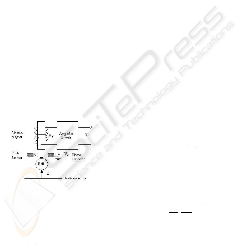
3 APPLICATION TO THE

MODEL OF A MAGNETIC

LEVITATION SYSTEM

In this work we consider the single-axis levitation

system described in (Cho et al., 1993) (see Fig. 1).

A force balance analysis leads to a state space rep-

resentation of the system with state x = (x

) =

(d − d

d −

) and control input u = V

−V

where

d is the the distance of the ball from the reference line

and V

is the control voltage applied to the ampliﬁer;

and

are equilibrium points for a given nominal

control voltage V

. The state space representation is

given by

˙x = f(x) + g(x)u, y = h(x) = x

(12)

with

f(x) =



b(x

/m− g



, g(x) =



b(x

)/m



(13)

where m is the mass of the ball, g is the gravity

and

b(x

) = 1/[a

− d

)

+ a

− d

) + a

], with

, a

and a

being real constant parameters. Since

h(x) =

b(x

)/m 6= 0, the system has a relative de-

gree r = 1 . Thus, in the coordinates ξ = (y,z) =

), the levitation system (12),(13) takes the form

˙y = [

b(z)V

/m− g] + [

b(z)/m]u,

˙z = y.

(14)

Figure 1: Schematic diagram of the magnetic levitation sys-

tem.

The system’s zero dynamics are then described

by the ﬁrst order differential equation ˙z = f

∗

(z) =

0 for which the quadratic positive deﬁnite function

∗

(z) = (1/2)z

satisﬁes L

∗

(z) = 0, and the sys-

tem is weakly minimum phase. One then has that the

feedback

u =

b(z)

[−

b(z)

+ g− z+ w] (15)

makes the system (14) feedback equivalent to a C

passive system from w to y with a C

storage func-

tion V = W

∗

(z) + (1/2)y

. Even more, the resultant

closed-loop system is a loosless one because of the

fact that

V = yw. One can also verify that this closed-

loop system is zero-state observable, thus the addi-

tional feedback

w = −ky, (16)

with k > 0, can make the origin (y, z) = (0,0) of the

system

ξ =



˙y

˙z



F(ξ) =



−k −1

1 0



ξ =

Aξ. (17)

asymptotically stable.

In (Cho et al., 1993) it is noticed that the solenoid

characteristics change with temperature, and a change

of ±20% can appear in

b(x

) when the levitation sys-

tem has been operated for a short period of time.

Thus, the actual force-distance relationship, denoted

by b(d), may be expressed as

b(d) =

b(d) + ∆

b(d) (18)

where ∆

b(d) is an unknown modeling error which can

be as high as 20% of

b(d). The uncertain model asso-

ciated to the nominal model (14) can then be written,

also in the coordinates ξ = (y,z), as

˙y = [

b(z)V

/m− g] + [∆

b(z)V

/m]

+([

b(z)/m] + [∆

b(z)/m])u,

˙z = y.

(19)

This is, the uncertainties are given by ∆a(y,z) =

∆

b(z)V

/m and ∆b(y,z) = ∆

b(z)/m.

The switching function S(y,v) is given by (3) with

v = −z+ w. Such a choice leads to the control law

u = u

slid

b(z)

[−Γsign(S) −

b(z)

+ g− z+ w],

(20)

with Γ > 0, which allows to reach the sliding surface

in a ﬁnite time. By selecting the additional output

feedback (16), we obtain the closed-loop system

ξ =

Aξ+

G(ξ) (21)

where

G(ξ) =

(ξ) =







[−Γsign(S) +

∆

b(z)V

∆

b(z)

[

b(z)V

+ g− Γsign(S)

−z− ky]]







(22)

From the size of the modelling error ∆

b(z) one can

verify, after some computations, that the uncertainty

term

(ξ) satisﬁes the uniform bound ||

(ξ) ||≤ δ

for a constant δ. It then follows that the solution ξ(t)

of the uncertain system (21) is ultimately bounded for

t ≥ 0.

STABILIZATION OF UNCERTAIN NONLINEAR SYSTEMS VIA PASSIVITY FEEDBACK EQUIVALENCE AND

SLIDING MODE

341

The magnetic levitation system described by

equations (12),(13) was simulated together with the

passivity based sliding mode controller (3),(20). The

nominal value of the ball’s mass m and the con-

stant coefﬁcients used in the force-distance relation-

ship

b(z) were selected as in (Cho et al., 1993), this

is m = 2.206 gr, a

= 0.0231/mg, a

= −2.4455/mg,

= 64.58/mg. In fact, as it is noted in (Cho et al.,

1993), the validity of the

b(x

) is constrained to the

range of 35 mm and 48 mm. By choosing the nominal

value of the control applied to the ampliﬁer circuit to

beV

= 4.87 volts, we obtained the equilibrium point

) = (38.2 mm,0 mm/sec). The initial condi-

tions of the magnetic levitation system were ﬁxed to

(0) = 44.2 mm and x

(0) = 0 mm/sec, while the

controller parameters were selected as Γ = 10 and

k = 2. In order to diminish the effect of chattering

due to the discontinuity of the sign function, a satura-

tion function given by

sat(S) =







1, if S > ε

S/ε, if −ε ≤ S ≤ ε

−1, if S < −ε

with ε > 0, was used instead of the sign function.

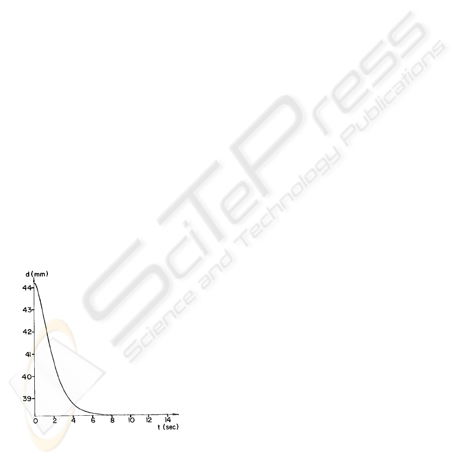
In order to evaluate the performance of the control

scheme, a variation of 20% in the value of the func-

tion

b(z) was introduced at t = 7 sec in all the simula-

tions. The time closed-loop plot corresponding to the

distance d is shown in Figures 2 for ε = 0.001. From

this plot, we can notice that the distance of the ball to

the reference line is always regulated to the equilib-

rium point d

= 38.2 mm with no overshoot.

Figure 2: Closed-loop response of the distance, d; ε =

0.001.

4 CONCLUSIONS

In this paper, a passivity-based sliding mode con-

troller design that allows to stabilize an uncertain non-

linear system has been presented. The proposed con-

troller has also been applied to the model of a mag-

netic levitation system in order to regulate the height

of a levitated ball around at one of its equilibria.

REFERENCES

Byrnes, C. I., Isidori, A., and Williams, J. C. (1991). Passiv-

ity, feedback equivalence, and the global stabilization

of minimum phase nonlinear systems. In IEEE Trans-

actions on Automatic Control, vol.36, pp. 1228-1240.

IEEE.

Cai, X. S. and Han, Z. Z. (2005). Inverse optimal con-

trol of nonlinear systems with structural uncertainty.

In IEE Proceedings Control Theory and Applications,

vol. 152, pp. 79-83. IEE.

Cho, D., Kato, Y., and Spilman, D. (1993). Sliding mode

and classical control of magnetic levitation systems.

In IEEE Control Systems, pp. 42-48. IEEE.

Duarte-Mermoud, M. A., Castro-Linares, R., and Castillo-

Facuse, A. (2002). Direct passivity of a class of mimo

non-linear systems using adaptive feedback. In Inter-

national Journal of Control, vol. 75, pp. 23-33. Taylor

and Francis.

Khalil, H. (1996). Nonlinear Systems. MacMillan Publish-

ing Company, New York, 2nd edition.

Loria, A., Panteley, E., and Nijmeier, H. (2001). A remark

on passivity-based and discontinuous control of un-

certain nonlinear systems. In Automatica, vol.37, pp.

1481-1487. Elsevier.

Mahmoud, M. S. and Zribi, M. (2002). Passive control

synthesis for uncertain systems with multiple-state

delays. In Computers and Electrical Enginnering,

vol.28, pp. 195-216. Pergamon.

Ortega, R. (1991). Passivity properties for stabilizing of

cascaded nonlinear systems. In Automatica, vol. 27,

pp. 423-424. Elsevier.

Su, W. and Xie, L. (1998). Robust control of nonlinear feed-

back passive systems. In Systems Control Letters, vol.

28, pp. 85-93. Elsevier.

Tunay, I. and Kaynak, O. (1995). A new variable struc-

ture controller for afﬁne nonlinear systems with non-

matching uncertainties. In International Journal of

Control, vol. 62, pp. 917-939. Taylor and Francis.

Utkin, V. I. (1992). Sliding Modes in Control and Optimiza-

tion. Springer, New York, 1st edition.

ICINCO 2007 - International Conference on Informatics in Control, Automation and Robotics

342