
MODIFIED MODEL REFERENCE ADAPTIVE CONTROL FOR
PLANTS WITH UNMODELLED HIGH FREQUENCY DYNAMICS
L. Yang, S. A. Neild and D. J. Wagg
Department of Mechanical Engineering, University of Bristol, Queens Building, University Walk, Bristol BS8 1TR, U.K.
Keywords:
Model reference adaptive control, Robustness, Unmodelled dynamics, Frequency response technique.
Abstract:
In this paper we develop a modified MRAC strategy for use on plants with unmodelled high frequency dy-
namics. The MRAC strategy is made up of two parts, an adaptive control part and a fixed gain control part.
The adaptive algorithm uses a combination of low and high pass filters such that the frequency range for the
adaptive part of the strategy is limited. This reduces adaptation to unexpected high frequency dynamics and
removes low frequency gain wind-up. In this paper we consider two examples of plants with unmodelled high
frequency dynamics, both of which exhibit unstable behaviour when controlled using the standard MRAC
strategy. By using the modified strategy we demonstrate that robustness is significantly improved.
1 INTRODUCTION
Two of the major challenges in the application of
model reference adaptive control (MRAC) strategies
are disturbances and plant uncertainty (Astr
¨
om and
Wittenmark, 1995; Sastry and Bodson, 1989; Landau,
1979; Popov, 1973). One effect of disturbances, such
as transducer noise, is that control gains can ‘wind-
up’ (Ioannou and Kokotovic, 1984; Virden and Wagg,
2005). An effective way to remove gain wind-up be-
haviour is to eliminate the inherent zero eigenvalue in
the (localised) MRAC system by introducing a com-
plementary low pass filter (Yang et al., 2006). Plants
with unmodelled high frequency dynamics are one
important case of plant uncertainty, and previous stud-
ies have shown how this can cause system instability
in many real applications (Rohrs et al., 1985; Nikzad
et al., 1996; Crewe, 1998; Neild et al., 2005b).
As an example of using MRAC on plants with
higher order unmodelled dynamics, we consider the
application of the MRAC to hydraulic shaking tables.
Hydraulic shaking tables are widely used in the earth-
quake engineering community for dynamic testing of
structures subjected to extreme loading. Adaptive
control is desirable due to the changing dynamics of
the test specimen attached to the table when exposed
to extreme loading (Stoten and G
´
omez, 2001). Gen-
erally hydraulic actuators may be modelled as first or-
der systems (Neild et al., 2005a), however attaching a
large mass, such as the table and payload, to the actu-
ator can lead to significant higher frequency dynam-
ics due to oil column resonance (Nikzad et al., 1996;
Crewe, 1998; Neild et al., 2005b).
In this paper we present a modified MRAC algo-
rithm which uses complementary filters at both low
and high frequency. We demonstrate that when this
new modified MRAC algorithm is applied to systems
with unmodelled high frequency dynamics a stable re-
sponse can be achieved.
2 FORMULATIONS OF
MODIFIED MRAC STRATEGY
In this section a brief introduction of ρ/φ modified
MRAC algorithm is given for a single-input single-
output (SISO) system. For more detailed discussions
of standard MRAC can be found in (Landau, 1979;
Sastry and Bodson, 1989; Astr
¨
om and Wittenmark,
1995). The system studied in this paper is based
on a first-order linear plant approximation given by
the transfer function G(s) = X(s)/U(s) = b/(s+ a),
where X(s) is the plant state (x(t) in the time domain),
196
Yang L., A. Neild S. and J. Wagg D. (2007).
MODIFIED MODEL REFERENCE ADAPTIVE CONTROL FOR PLANTS WITH UNMODELLED HIGH FREQUENCY DYNAMICS.
In Proceedings of the Fourth International Conference on Informatics in Control, Automation and Robotics, pages 196-201
DOI: 10.5220/0001617101960201
Copyright
c
SciTePress

U(s) is the control signal and a and b are the plant pa-
rameters. The control signal is generated from the
state variable and the reference (or demand) signal
r(t), using adaptive control gains K and K
r
, such
that u(t) = Kx(t) + K
r
r(t), where K is the feedback
adaptive gain and K
r
the feed forward adaptive gain.
The plant is controlled to follow the output from a
reference model G
m
(s) = X
m
(s)/R(s) = b
m
/(s+a
m
),
where X
m
is the state of the reference model and a
m
and b
m
are the reference model parameters which are
specified by the controller designer. The block dia-
gram of MRAC is illustrated by Fig.1.
K
Reference Model
G
m
=b
m
/(s+a
m
)
Adaptive
Algorithm
+
+
K
r
+
-
C
e
x
m
r
u=K*x+K
r
*r
x
y
e
Plant
G=b/(s+a)
X
e
Figure 1: Schematic block diagram of the model reference
adaptive control system. K and K
r
are the adaptive gains
generated using the MRAC algorithm.
The object of the MRAC algorithm is for x
e
→ 0
as t → ∞, where x
e
= x
m
− x is the error signal. The
dynamics of the system can be rewritten in terms of
the error such that
˙x
e
= (−a+bK)x
e
+ b(K
E
− K)x
m
+ b(K
E
r
− K
r
)r,
(1)
where K
E
and K
E
r
are Erzberger gains. The Erzberger
gains are defined as the linear gains which results in
the plant response matching the reference model re-
sponse (Khalil, 1992);
K
E
=
a− a
m
b
, K
E
r
=
b
m
b
. (2)
For general model reference adaptive control, the
adaptive gains are commonly defined by using Hyper-
stability rule (Popov, 1973), which is a proportional
plus integral formulation
K(t) = α
t
0
C
e
x
e
x(τ)dτ+ βC
e
x
e
x(t) + K
0
,
K
r
(t) = α
t
0
C
e
x
e
r(τ)dτ + βC
e
x
e
r(t) + K
r0
,
(3)
where α and β are adaptive control weightings rep-
resenting the adaptive effort and K
0
and K
r0
are the
initial gain values. In the case of a first-order imple-
mentation, C
e
is a scalar and therefore may be incor-
porated into the α and β adaptive control weightings.
2.1 Mrac with ρ Modification
The purpose of introducing the ρ modification to the
MRAC algorithm is to resolve the problem of gain
‘wind-up’ observed using standard the MRAC strat-
egy on plants with output disturbances. The modified
adaptive gains K
mρ
and K
rmρ
are given by
K
mρ
(s) =
s
s+ρ
2
K(s) +
ρ
2
s+ρ
2
K
∗
(s),
K
rmρ
(s) =
s
s+ρ
2
K
r
(s) +
ρ
2
s+ρ
2
K
∗
r
(s),
(4)
where ρ is a constant, K(s) and K
r
(s) are the stan-
dard adaptive control gains in the Laplace domain,
and K
∗
(s) and K
∗
r
(s) are constant gains. This mod-
ification eliminates a zero eigenvalue in the localised
error dynamics about the equilibrium point, replacing
it with an eigenvalue of −ρ
2
, hence making all the
system eigenvalues asymptotically stable (Yang et al.,
2006). The ρ modified MRAC can also be explained
in terms of frequency response. A bode plot of Eq.4 is
shown in Fig.2(a), we can see how the ρ term works as
a low frequency filter on the adaptive gains and stops
gain wind-up by pushing gains to fixed values. Ex-
perimental tests have demonstrated the effectiveness
of ρ modified MRAC on preventing gain wind-up in
a small scale motor-driven shaking table (Yang et al.,
2006).
2.2 Mrac with ρ/φ Modification
In this paper we present an additional modification
to MRAC through the use of an additional high fre-
quency complementary filter. A φ term is introduced
as the complementary filter to reduce adaptation to
high frequencies, e.g. due to the unmodelled dynam-
ics. This is illustrated in Fig.2(b).
The ρ/φ modified MRAC control gains may be de-
scribed in the Laplace domain as
K
m
(s) =
φ
2
s
(s+ρ
2
)(s+φ
2
)
K(s) +
ρ
2
s+ρ
2
K
∗
(s)
+
s
2
(s+ρ
2
)(s+φ
2
)
K
∗
(s),
K
rm
(s) =
φ
2
s
(s+ρ
2
)(s+φ
2
)
K
r
(s) +
ρ
2
s+ρ
2
K
∗
r
(s)
+
s
2
(s+ρ
2
)(s+φ
2
)
K
∗
r
(s),
(5)
where ρ and φ are constants which need to be se-
lected by the designer, and K
∗
and K
∗
r
are steady-
state gains, ideally they are set to the values of the
Erzberger Gains. K and K
r
are the standard MRAC
control gains.
By inspecting Eq.5, we note that the modified con-
trol gain K
m
is made up of an adaptive part and a fixed
MODIFIED MODEL REFERENCE ADAPTIVE CONTROL FOR PLANTS WITH UNMODELLED HIGH
FREQUENCY DYNAMICS
197

10
−4
10
−3
10
−2
10
−1
10
0
10
1
10
2
10
3
10
4
−40
−20
0
20
(a) Bode Diagram
Frequency (rad/sec)
Magnitude (dB)
10
−4
10
−3
10
−2
10
−1
10
0
10
1
10
2
10
3
10
4
−40
−20
0
20
(b) Bode Diagram
Frequency (rad/sec)
Magnitude (dB)
Figure 2: (a) ρ modified MRAC adaptive gain structure.
Solid line represents the fixed gain control part, K
∗
or K
∗
r
,
and dash-dot line represents gains adaptive part, K or K
r
.
The vertical dash line shows the value of ρ
2
corresponding
to the complementary filters break point. (b) ρ and φ mod-
ified MRAC structure. Solid line represents the fixed gain
control part K
∗
or K
∗
r
, and dash-dot line represents gains
adaptive part K or K
r
. Vertical dash line shows the value of
ρ
2
and φ
2
.
gain control part. The first term on the right hand side
is the adaptive part, and the second and third terms are
fixed gain control terms based on the constant steady-
state gain K
∗
(s). The same situation can be found in
the modified gain K
rm
. Given ρ and φ are non-zero
real values, the fixed gain part of Eq.5 has all poles on
left half plane, hence this part is stable. Now we focus
on the stability of the adaptive part of modified con-
trol gains. By applying the Laplace transform given
zero initial conditions to Eq. 3 we have
K(s) − K
0
P
1
(s)
=
βs+ α
s
,
K
r
(s) − K
r0
P
2
(s)
=
βs+ α
s
, (6)
where P
1
(s) = C
e
X
e
(s)X(s) and P
2
(s) = C
e
X
e
(s)R(s).
We note that a zero pole exists which makes the trans-
fer function marginally stable. Substituting K(s) and
K
r
(s) in Eq.5 by Eq.6, the adaptive part of Eq.5 be-
comes
K
m
(s)−K
0
P
1
(s)
=
φ
2
(βs+α)
(s+ρ
2
)(s+φ
2
)
,
K
rm
(s)−K
r0
P
2
(s)
=
φ
2
(βs+α)
(s+ρ
2
)(s+φ
2
)
.
(7)
Comparing Eq.7 with standard MRAC control gains
of Eq.6, we noticed that the zero pole in the standard
MRAC control gain is replaced by two negative poles,
given ρ and φ are non-zero real values, and this makes
the control gains asymptotically stable.
Now we consider the overall transfer function path
from the input signal r to error signal e. Given plant
transfer function G and reference model transfer func-
tion G
m
, the transfer function from reference signal r
to plant output x can be written as (Astr
¨
om and Wit-
tenmark, 1995)
G
c
(s) =
X(s)
R(s)
=
K
r
G
1− KG
. (8)
So the error signal x
e
becomes X
e
(s) = [G
m
(s) −
G
c
(s)]R(s), hence the transfer function from refer-
ence signal r to error signal x
e
can be written as
X
e
(s)/R(s) = G
m
− G
c
, substituting G
c
(s) by Eq.8 and
rearranging it we have
X
e
(s)
R(s)
=
G
m
− KG
m
G− K
r
G
1− KG
. (9)
Since the transfer function of plant is G(s) = b/(s+
a) and the transfer function of reference model is
G
m
(s) = b
m
/(s+ a
m
), Eq.9 can be calculated as
X
e
(s)
R(s)
=
b(K
E
r
− K
r
)s+ b
m
b(K
E
− K) + a
m
b(K
E
r
− K
r
)
(s+ a
m
)(s+ a− bK)
.
(10)
Eq.10 represents the error response of the overall sys-
tem. We notice there are two poles −a
m
and bK − a
in this transfer function. To make the overall system
stable, we need to ensure both poles are on left half
plane. Since a
m
is defined as positive, the −a
m
pole
is on left-half plane. To make bK − a < 0, the con-
dition of K < a/b need to be satisfied. We notice if
K = K
E
= (a − a
m
)/b this condition will always be
satisfied.
As a further insight into Eq.5 and Eq.10, if ρ = ∞
and φ = 0, Eq.5 will become K
m
= K
∗
and K
rm
= K
∗
r
,
which means the system will be completely controlled
by fixed gains. Hence to increase ρ from 0 and de-
crease φ from infinite means to add weights on fixed
gain control. In Eq.10 if K = K
∗
= K
E
r
and K
r
= K
∗
r
=
K
E
r
the error signal will become zero, which means
the system has ideal response. We therefore set K
∗
and K
∗
to our best estimate of the Erzberger gains K
E
and K
E
r
.
3 MODIFIED MRAC APPLIED TO
ROHRS EXAMPLE
Knowledge of the Erzberger gains, to set K
∗
and
K
∗
, is important to the accuracy to the ρ/φ modified
MRAC algorithm. In many practical situations the
Erzberger Gains can not be estimated precisely and in
some cases can only be crudely approximated. One
such case is a plant with unmodelled high frequency
dynamics, for example ‘Rohrs model’ (Rohrs et al.,
1985). In this section we show how the modified
MRAC algorithm copes with Rohrs example. The
plant transfer function is given as
G(s) =
2
(s+ 1)
229
(s
2
+ 30s+ 229)
, (11)
ICINCO 2007 - International Conference on Informatics in Control, Automation and Robotics
198

which is a nominally first order plant 2/(s + 1)
multiply by a second order unmodelled dynamics
229/(s
2
+30s+229) which has almost critical damp-
ing, ζ = 1.02. The plant thus has two poles s =
−15 ± 2i neglected in the model used to design the
adaptive controller. The reference model is given as
G
m
(s) =
3
s+ 3
. (12)
The initial conditions for both control gains K and K
r
are zero. As in Rohrs example the input signal is set
as
r(t) = 0.3+ 1.85sin(16.1t), (13)
much higher frequency than the nominal first order
plant break frequency (1 rad/sec). Nominal Erzberger
gains can be calculated according to Eq.2 as K
E
= −1
K
E
r
= 1.5. The α/β ratio is chosen as 1, which is the
same as nominal plant break frequency.
0 5 10 15 20
−5
0
5
Output x
0 5 10 15 20
0
10
20
K
r
0 5 10 15 20
−40
−20
0
Time
K
Figure 3: Standard MRAC with unmodelled dynamics
(Rohrs model), input signal r(t)=0.3+1.85sin(16.1t), α =
β = 1. The system is unstable.
If the standard MRAC strategy is applied to the
nominal first order plant, G = 2/(s+ 1), the response
is stable and the gains tend to the Erzberger values.
However if the higher frequency dynamics, as de-
scribed by Eq.11 are included in the plant gain wind-
up occurs which results in system instability. Fig.3
shows the system response with α = β = 1 , which
results in system instability within 25 seconds.
Fig.4 shows the plant response, for the case where
with high frequency dynamic are included, using ρ
modified MRAC, ρ
2
= 0.4 and α = β = 1. The mod-
ified strategy results in a stable response with no gain
wind-up.
0 5 10 15 20 25 30 35 40 45 50
−1
0
1
Output x
0 5 10 15 20 25 30 35 40 45 50
0
2
4
K
r
0 5 10 15 20 25 30 35 40 45 50
−4
−2
0
Time
K
Figure 4: ρ modified MRAC with Rohrs model, input signal
r(t)=0.3+1.85sin(16.1t), α = β = 1, ρ
2
= 0.4. The system is
stable.
4 MODIFIED MRAC APPLIED TO
SHAKING TABLES
In this section, to demonstrate the difference in be-
haviour due to the ρ and the φ modifications, we con-
sider the application of the MRAC strategy to con-
trol hydraulic shaking tables. Under general operat-
ing conditions, a large hydraulic shaking table used
for earthquake tests will have a low frequency demand
which is affected by high frequency dynamics due to
oil column resonance. Typically system identification
of hydraulic shaking tables over the low frequency
operating range, around 0-10 Hz, results in a first or-
der approximation to the system dynamics with the
break frequency occurring within the operating range.
However oil column resonance causes an unmodelled
high frequency resonance with low damping, in the
order of 10% of critical damping, (Nikzad et al., 1996;
Crewe, 1998; Neild et al., 2005b).
To simulate this type of application, we will make
the following changes to Rohrs example considered in
the last section. Firstly, we change the demand signal
frequency to 1 rad/sec, such that it coincides with the
nominal plant break frequency:
r(t) = 0.3+ 1.85sin(1t). (14)
Secondly, we add white Gaussian noise to the plant
output, resulting in an approximate signal to noise
ratio of 20, to mimic transducer noise. Thirdly, we
change the damping ratio of the higher frequency un-
modelled dynamics to ζ = 0.1 to represent the oil col-
umn resonance to give the overall plant transfer func-
tion:
G(s) =
2
(s+ 1)
229
(s
2
+ 3s+ 229)
, (15)
MODIFIED MODEL REFERENCE ADAPTIVE CONTROL FOR PLANTS WITH UNMODELLED HIGH
FREQUENCY DYNAMICS
199
where the nominal first order plant is still 2/(s + 1),
but the unmodelled dynamics becomes 229/(s
2
+
3s + 229). A Bode plot of the plant is given in
Fig.5(a). The reference model and other conditions
remain unaltered.
10
−2
10
−1
10
0
10
1
10
2
−60
−40
−20
0
(a) Bode Diagram
Frequency (rad/sec)
Magnitude (dB)
10
−2
10
−1
10
0
10
1
10
2
−60
−40
−20
0
(b) Bode Diagram
Frequency (rad/sec)
Magnitude (dB)
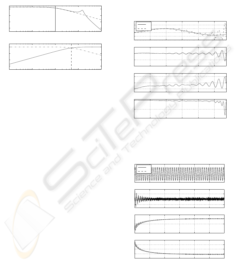
Figure 5: (a) Plant dynamics Bode plot: solid line shows the
plant with unmodelled high frequency dynamics, the dash
line is the nominal first order plant and the vertical line rep-
resents input signal operating frequency 1 rad/sec. (b) φ
modified MRAC: dash-dot line represents adaptive part of
the control gains K or K
r
, solid line represents the fix part
K
∗
or K
∗
r
and the vertical dash line represents the φ comple-
mentary filter break frequency; φ
2
= 5 rad/sec.
As with Rohrs example, the standard MRAC strat-
egy exhibits gain windup resulting in system instabil-
ity when applied to the plant with higher frequency
dynamics.
Fig.6 shows the control performance using ρ mod-
ified MRAC (with ρ
2
= 0.5 and α = β = 0.5). We
can see that, in contrast to Rohrs example, this sys-
tem is still unstable despite the ρ modification. This
is because the ρ modification is designed to remov-
ing windup rather than the gain oscillations that occur
when the unmodelled higher order dynamics has low
damping.
Fig.7 is the system response using the φ modified
MRAC algorithm (with φ
2
= 5 and α = β = 0.5). The
value of φ has been selected to reduce gain adaptation
at the oil column resonance frequency of 11 rad/sec.
The system is stable, with the error and both gains
settle around 150 seconds. Comparing Fig.7 with
Fig.6, we observe that φ plays a different role from
ρ in the modified control algorithm. The φ modifica-
tion results in filtering out the unmodelled high fre-
quency dynamics directly to avoid the system adapt-
ing to these undesirable dynamics. In this example
setting φ
2
= 5 can minimise the gain adaptation to the
oil column resonance, as illustrated by Fig.5(b) which
shows the resulting complementary filters applied to
the adaptive, K, and linear, K
∗
, gains.
Finally, Fig.8 shows the control result using the
combined ρ/φ modified MRAC algorithm (with α =
β = 0.5, ρ
2
= 0.5 and φ
2
= 5). The system has a stable
response, with the error and gains settle within around
10 seconds – faster than when φ modified MRAC was
used. The reason is that by increasing ρ the fixed gain
contribution to the controller, which requires no time
to settle, becomes more dominant.
0 1 2 3 4 5
−4
−2
0
2
4
6
Output
x
m
x
0 1 2 3 4 5
−10
−5
0
5
error
0 1 2 3 4 5
0
2
4
K
r
0 1 2 3 4 5
−20
−10
0
Time
K
Figure 6: Plant with unmodelled high frequency dynamics,
damping ratio 0.1, controlled by ρ modified MRAC. Input
signal r(t)=0.3+1.85sin(1t), α = β = 0.5, ρ
2
= 0.5. System
is unstable.
0 50 100 150 200 250 300
−2
0
2
Output
x
m
x
0 50 100 150 200 250 300
−0.5
0
0.5
error
0 50 100 150 200 250 300
0
1
2
K
r
0 50 100 150 200 250 300
−1.5
−1
−0.5
0
0.5
Time
K
Figure 7: Plant with unmodelled high frequency dynamics,
damping ratio 0.1, controlled by φ modified MRAC. Input
signal r(t)=0.3+1.85sin(1t), α = β = 0.5, φ
2
= 5. System is
stable. Error and gains settle within around 150 seconds.
ICINCO 2007 - International Conference on Informatics in Control, Automation and Robotics
200

0 10 20 30 40 50 60 70 80 90 100
−2
0
2
Output
x
m
x
0 10 20 30 40 50 60 70 80 90 100
−0.4
−0.2
0
0.2
0.4
error
0 10 20 30 40 50 60 70 80 90 100
0
1
2
K
r
0 10 20 30 40 50 60 70 80 90 100
−1.5
−1
−0.5
0
Time
K
Figure 8: Plant with unmodelled high frequency dynamics,
damping ratio 0.1, controlled by ρ/φ modified MRAC. Input
signal r(t)=0.3+1.85sin(1t), α = β = 0.5, ρ
2
= 0.5, φ
2
= 5.
System is stable. Error and gains settle within around 10
seconds.
5 CONCLUSION
In this paper we have introduced a ρ/φ modified
MRAC strategy and tested it on plants with unmod-
elled high frequency dynamics. The modified MRAC
strategy is made up of two parts, an adaptive control
part and a fix gain control part. In the frequency do-
main, the ρ and φ modifications are first-order com-
plementary filters which replace the adaptive gain
with a fixed gain at low and high frequency respec-
tively. Two types of unmodelled high frequency dy-
namics are considered. Firstly using Rohrs model,
in which the unmodelled dynamics are almost critical
damped, it was observed that ρ modified MRAC elim-
inated the gain wind-up. Secondly when the plant has
lightly damped unmodelled dynamics case, similar
to the oil column dynamics observed with hydraulic
shaking table control, using φ modified MRAC pre-
vents the system adapting to unmodelled high fre-
quency dynamics, hence stabilizing the system. Sim-
ulation results show that φ modification results in fil-
tering off the unmodelled high frequency dynamics
directly to avoid the system adapting to these undesir-
able dynamics whereas the ρ modification eliminates
gain wind-up. Hence the ρ/φ modified MRAC is a ef-
fective way to control systems with unmodelled high
frequency dynamics.
ACKNOWLEDGEMENTS
The authors would also like to acknowledge the
support of the EPSRC. Lin Yang is supported by
the Dorothy Hodgkin Postgraduate Award scheme
(EPSRC-BP) and David Wagg by an Advanced Re-
search Fellowship.
REFERENCES
Astr
¨
om, K. J. and Wittenmark, B. (1995). Adaptive control.
Addison-Wesley, second edition.
Crewe, A. (1998). The Characterisation and Optimisation
of Earthquake Shaking Table Performance. PhD the-
sis, University of Bristol.
Ioannou, P. and Kokotovic, P. (1984). Instability analysis
and improvement of robustness of adaptive control.
Automatica, 20(5):583–594.
Khalil, H. (1992). Nonlinear Systems. Macmillan:New
York.
Landau, Y. (1979). Adaptive control:The model reference
approach. Marcel Dekker:New York.
Neild, S., Drury, D., and Stoten, D. (2005a). An im-
proved substructuring control strategy based on the
mcs control algorithm. Proceedings of the I. Mech. E.
Part I, Journal of Systems and Control Engineering,
219(5):305–317.
Neild, S., Stoten, D., Drury, D., and Wagg, D. (2005b).
Control issues relating to real-time substructuring ex-
periments using a shaking table. Earthquake Engi-
neering and Structural Dynamics, 34(9):1171–1192.
Nikzad, K., Ghaboussi, J., and Paul, S. (1996). Actua-
tor dyanamics and delay compensation using neuro-
controllers. Journal of Engineering Mechanics, 122-
10:966–975.
Popov, V. (1973). Hyperstability of control systems.
Springer.
Rohrs, C., Valavani, L., Athans, M., and Stein, G. (1985).
Robustness of continuous-time adaptive control algo-
rithms in the presence of unmodeled dynamics. IEEE
Trans. Automat. Contr, AC-30:881–889.
Sastry, S. and Bodson, M. (1989). Adaptive control : Stabil-
ity, convergence and robustness. Prentice-Hall : New
Jersey.
Stoten, D. and G
´
omez, E. (2001). Real-time adaptive
control of shaking tables using the minimal control
synthesis algorithm. Phil. Trans. R Soc. Lond. A.,
359:1697–1723.
Virden, D. and Wagg, D. (2005). System identification of
a mechanical system with impacts using model refer-
ence adaptive control. Proc. IMechE. Pat I: J. Syst.
Control Eng., 219:121–132.
Yang, L., Neild, S., Wagg, D., and Virden, D. (2006). Model
reference adaptive control of a nonsmooth dynamical
system. Nonlinear Dynamics, 46(3):323–335.
MODIFIED MODEL REFERENCE ADAPTIVE CONTROL FOR PLANTS WITH UNMODELLED HIGH
FREQUENCY DYNAMICS
201
