
SATURATION FAULT-TOLERANT CONTROL FOR LINEAR
PARAMETER VARYING SYSTEMS
Ali Abdullah
Kuwait University, Electrical Engineering Department, P. O. Box 5969, Safat-13060, Kuwait
Keywords:
Fault diagnosis, fault-tolerant systems, parameter estimation.
Abstract:
This paper presents a methodology for designing a fault-tolerant control (FTC) system for linear parameter
varying (LPV) systems subject to actuator saturation fault. The FTC system is designed using linear matrix
inequality (LMI) and model estimation techniques. The FTC system consists of a nominal control, fault
diagnostic, and fault accommodation schemes. These schemes are designed to achieve stability and tracking
requirements, estimate a fault, and reduce the fault effect on the system. Simulation studies are used to
illustrate the proposed design.
1 INTRODUCTION
In recent years, the field of designing FTC systems
has received considerable attention (Blanke et al.,
2001; Bodson, 1995; Isermann et al., 2002; Patton,
1997; Rauch, 1994; Stengel, 1991). For the case of
actuator fault, most of this research had addressed
fault accommodation for system subject to parame-
ter variation or frozen output. Other types of actua-
tor fault have been rarely considered. In this paper,
a methodology for designing FTC system for LPV
systems subject to a reduction in the actuator satura-
tion limit is presented. The LPV systems are defined
as a class of linear time-varying systems whose state
space matrices depend on a set of parameters that are
bounded and can be measured or estimated online.
In the case of using an analytical approach, the main
idea behind fault tolerance is the use of fault diagnos-
tic and accommodation schemes. A fault diagnostic
scheme driven by plant measurements is used to de-
tect, locate, and estimate faults; while a fault accom-
modation scheme driven by fault information from the
diagnostic scheme is used to modify the nominal con-
trol law in order to reduce the fault effect on the sys-
tem. Based on the above idea, the total task of the
proposed FTC system is divided into three parts:
• Plant control: attempts to stabilize the closed-loop
system and provide the desired tracking properties
in the absence of faults. The controller is designed
using LPV technique (Apkarian et al., 1995; Ap-
karian and Adams, 1998; Gahinet et al., 1996;
Kose et al., 1998; Tuan and Apkarian, 2002).
• Fault diagnosis: deals with the problem of satura-
tion fault detection, location, and level estimation.
To achieve that, a suitable LPV model is derived
to describe the faulty system. Then the results in
(Polycarpou and Helmicki, 1995) are used to con-
struct the diagnostic scheme.
• Fault accommodation: attempts to reduce the fault
effect on the system by modifying the nominal
control law through the reference reshaping fil-
ter and feed-forward gain. The accommodation
scheme is designed with the help of the bounded
real lemma for LPV system presented in (Gahinet
et al., 1996).
The notation
H (A ,B ,C ,D ,E ,F ) is used through-
out the paper to denote the symmetric matrix
A B C
B
T
D E
C
T
E
T
F
.
19
Abdullah A. (2007).
SATURATION FAULT-TOLERANT CONTROL FOR LINEAR PARAMETER VARYING SYSTEMS.
In Proceedings of the Fourth International Conference on Informatics in Control, Automation and Robotics, pages 19-24
Copyright
c
SciTePress

2 PROBLEM STATEMENT
Consider a class of LPV systems of the form:
˙x
s
(t) = A
s
(ρ(t))x
s
(t) + B
s
u(t) (1)
y(t) = x
s
(t) (2)
where x
s
(t) ∈ ℜ
n
is the state vector, u(t) ∈ ℜ
m
is the
control signal, and y(t) ∈ ℜ
n
is the measured output
signal. A
s
(ρ(t)) = A
s
o
+
∑
N
i=1
ρ
i
(t)A
s
i
, and A
s
j
and B
s
are known constant matrices with appropriate dimen-
sions. Furthermore, ρ(t) = (ρ
1
(t),... , ρ
N
(t))
T
is the
vector of real time varying parameters ranging inside
the hyper-rectangle region defined by ρ
i
(t) ∈ [ρ
i
,
¯
ρ
i
].
Also, its rate
˙
ρ(t) = (
˙
ρ
1
(t),... ,
˙
ρ
N
(t))
T
is ranging
inside another hyper-rectangle region defined by
˙
ρ
i
(t) ∈ [ν
i
,
¯
ν
i
].
The actuator saturation fault considered in this
study is given by Definition 1.
Definition 1 (Actuator Saturation Fault) The ac-
tuator saturation fault is defined mathematically as:
σ
j
(δ
j
u
j
) =
u
j
|u
j
| < δ
j
¯u
j
δ
j
¯u
j
sign(u
j
) |u
j
| ≥ δ
j
¯u
j
where u
j
is the input to the jth actuator, σ
j
is the out-
put of the jth actuator, and 0 ≤ δ
j
≤ 1 is the reduced
level of the jth saturation limit ¯u
j
.
Remark 1 The value of δ
j
represents the reduced
level of the actuator saturation limit where δ
j
= 0
means a complete failure, δ
j
= 1 means no failure ex-
ists, and 0 < δ
j
< 1 means the saturation limit has
been reduced to the value of ±δ
j
¯u
j
.
Now the main problem is presented.
Problem 1 Design an FTC system for the LPV sys-
tem (1)-(2) such that:
• In the absence of actuator saturation fault, the
nominal control objectives are achieved.
• In the presence of actuator saturation fault, the
control objectives are achieved as close as possi-
ble to the nominal one.
3 FAULT-TOLERANT CONTROL
SYSTEM
The main schemes of the FTC system are shown in
Figure 1. These schemes are controller, fault diag-
nosis, and fault accommodation. Furthermore, the
fault accommodation scheme consists of reconfigura-
tion mechanism, feed-forward gain, and reference re-
shaping filter. The controller is designed to achieve
System
Fault
Diagnosis
Controller
+
Reference
Signals
Inputs
Outputs
Reshaped
Reference
Signals
Fault
Information
Fault
Accommodation
Fault
Reconfiguration
Mechanism
Feed-Forward
Gain
Reshaping
Filter
Figure 1: Structure of fault-tolerant control system.
the desired system performances assuming that the
system is under normal operation. The fault diag-
nostic scheme is designed to detect, locate, and es-
timate a fault. The fault diagnostic scheme is driven
by the available system input and output signals. The
fault information (no fault, fault, location and magni-
tude of fault) is supplied to the reconfiguration mech-
anism to trigger an appropriate reconfiguration of the
feed-forward gain and reference reshaping filter. The
feed-forward gain and reference reshaping filter are
designed to fulfill the new physical constraints im-
posed by the fault.
3.1 Control Design
The controller is designed based on the concept of
affine quadratic stability (Gahinet et al., 1996) defined
below.
Definition 2 (Affine Quadratic Stability) The LPV
system ˙x = A
c
(ρ)x is affinely quadratically stable
(AQS) if there exists N+1 symmetric matrices P
i
such
that the following inequalities:
P(ρ)= P
o
+ρ
1
P
1
+... + ρ
i
P
i
+... + ρ
N
P
N
>0 (3)
F(ρ,
˙
ρ)= A
c
(ρ)
T
P(ρ)+P(ρ)A
c
(ρ)+
dP(ρ)
dt
<0, (4)
where
dP(ρ)
dt
=
˙
ρ
1
P
1
+ ... +
˙
ρ
i
P
i
+ ... +
˙
ρ
N
P
N
, hold
for all admissible trajectories of the parameter vec-
tor ρ. In this case, the function V(x,ρ) = x
T
P(ρ)x
is a quadratic Lyapunov function for the LPV system
˙x = A
c
(ρ)x.
The difficulty associated with the control design us-
ing Definition 2 is that the matrix inequality (4) is
not linear in terms of P(ρ) and A
c
(ρ). However,
Lemma 1 (Bara et al., 2001) can be used instead of
Definition 2 to simplify a controller design.
Lemma 1 The LPV system ˙x(t) = A
c
(ρ)x(t) is AQS
if there exist a constant matrix W and a symmetric
matrix P(ρ) such that the following LMI:
H (−W −W
T
,W
T
A
c
(ρ)
T
+ P(ρ),W
T
,

−P(ρ) +
dP(ρ)
dt
,0,−P(ρ)) < 0 (5)
holds for all admissible trajectories of the parameter
vector ρ.
Since the parameter vector ρ ranges over a polytope,
the LMI (5) involves infinite number of constraints.
Theorem 1 is used to reduce the infinite number of
constraints into a finite one, hence simplifying the
controller design.
Theorem 1 If there exist matrices W, R
i
, and sym-
metric matrices P
i
such that the following LMIs:
H (−W −W
T
,(A
s
(Ve
i
)W − B
s
R
i
+ P(Ve
i
))
T
,W
T
,
−P(Ve
i
) − P
o
+ P(
˜
Ve
i
),0,−P(Ve
i
)) < 0 (6)
are feasible for all (Ve
i
,
˜
Ve
i
) where ρ =
∑
2
N
i=1
α
i
(t)Ve
i
,
and
˙
ρ =
∑
2
N
i=1
β
i
(t)
˜
Ve
i
with
∑
2
N
i=1
α
i
(t) = 1,
∑
2
N
i=1
β
i
(t) = 1, α
i
(t) ≥ 0, and β
i
(t) ≥ 0. Then,
the control law u = −(
∑
2
N
i=1
α
i
(t)K
i
)x(t) where
K
i
= R
i
W
−1
stabilizes the system (1)-(2).
Proof: is omitted.
To implement the control law u =
−(
∑
2
N
i=1
α
i
(t)K
i
)x(t), α
i
(t) must be available on-
line. α
i
(t) can be computed from the relation
ρ =
∑
2
N
i=1
α
i
(t)Ve
i
using the known Ve
i
and ρ(t).
3.2 Fault Diagnosis
To diagnosis a fault, consider the case where the sat-
uration limit of the jth actuator is reduced due to a
fault. Then, equation (1) is written as:
˙x
s
=A
s
(ρ)x
s
+B
s
1
u
1
... + B
s
j
σ
j
(δ
j
u
j
)... + B
s
m
u
m
(7)
For fault diagnosis, equation (7) is expressed in terms
of control outputs by defining:
λ
j
=
(
σ
j
(δ
j
u
j
)
u
j
− 1 u
j
6= 0
0 u
j
= 0
and then writing (7) as:
˙x
s
=
A
s
(ρ)x
s
(t) + B
s
u+ λ
j
B
s
j
u
j
u
j
6= 0
A
s
(ρ)x
s
+ B
s
u u
j
= 0
Theorem 2 is used to estimate the value of λ
j
which
will be used to detect the fault and to estimate the sat-
uration level δ
j
.
Theorem 2 Consider the estimated model:
˙
ˆx
s
= A
s
(ρ)x
s
+ B
s
u+
ˆ
λ
j
B
s
j
u
j
+ G( ˆx
s
− x
s
)
where ˆx
s
∈ R
n
is the estimated state vector, G is the
constant matrix with negative eigenvalues, and
ˆ
λ
j
∈ R
is the estimated parameter of λ
j
adjusted as:
˙
ˆ
λ
j
=Γ(B
s
j
u
j
)
T
e−χΓ
ˆ
λ
j
ˆ
λ
T
j
|
ˆ
λ
j
|
2
Γ(B
s
j
u
j
)
T
e;
ˆ
λ
j
(0) = 0 (8)
where e = x− ˆx is the estimated error, Γ is the posi-
tive definite matrix, and χ is the indicator function for
the projection algorithm (to prevent parameter drift)
defined as:
χ=
(
0 (|
ˆ
λ
j
|<M) or (|
ˆ
λ
j
|=Mand
ˆ
λ
T
j
Γ(B
s
j
u
j
)
T
e≤0)
1 (|
ˆ
λ
j
|=M and
ˆ
λ
T
j
Γ(B
s
j
u
j
)
T
e>0)
Then
ˆ
λ
j
is uniformly bounded, and lim
t−→∞
e(t) = 0.
Proof: is omitted.
For fault detection,
ˆ
λ
j
is tested for the likeli-
hood of saturation fault. A decision about the
existence of saturation fault is made as follows: if
ν
j
≤ ε
j
, the saturation fault doest not exist; if ν
j
> ε
j
,
the saturation fault exist. ν
j
= [
1
α
t+α
t
(
ˆ
λ
j
(τ))
2
dτ]
1/2
is the average energy of
ˆ
λ
j
over the time interval
[t,t + α], α is the detection window, and ε
j
is the
threshold.
For saturation level estimation, when the satura-
tion fault exists (i.e., ν
j
> ε
j
),
ˆ
λ
j
has the value:
ˆ
λ
j
=
σ
j
(
ˆ
δ
j
u
j
)
u
j
− 1 =
ˆ
δ
j
¯u
j
sign(u
j
)
u
j
− 1 =
ˆ
δ
j
¯u
j
|u
j
|
− 1.
Then the saturation level δ
j
can be estimated as:
ˆ
δ
j
=
|u
j
|
u
j
(
ˆ
λ
j
+ 1).
3.3 Fault Accommodation
To accommodate a saturation fault, a reference re-
shaping filter and feed-forward gain are used to ful-
fil the new input constraint |u
j
(t)| < δ
j
¯u
j
. To enforce
this constraint the jth system input u
j
(t) is generated
from the jth control output u
c
j
(t), which is a function
of a modified reference signal ¯r generated by the ref-
erence reshaping filter, and the jth feed-forward sig-
nal u
f
j
in order to get |u
j
(t) = u
c
j
(t) + u
f
j
(t)| < δ
j
¯u
j
.
Furthermore, the modified reference signal ¯r should
be designed to fulfil the input constraint while devia-
tion from the reference signal r is minimized. Based
on these suggestions, Problem 2 is addressed as fol-
lows.
Problem 2 Given the:
• System:
˙x
s
(t) = A
s
(ρ)x
s
(t) + B
s
u(t)
y(t) = x
s
(t)
• Controller:
˙x
c
(t)=A
c
(ρ)x
c
(t)+B
c
(ρ)¯r(t)+C
c
(ρ)x
s
(t)
u
c
(t)=D
c
(ρ)x
c
(t)+E
c
(ρ)¯r(t)+F
c
(ρ)x
s
(t)

• Saturation fault level: δ
j
Design a:
• Reference reshaping filter:
˙x
r
(t) = A
r
(δ
j
)x
r
(t) + B
r
(δ
j
)r(t)
¯r(t) = C
r
(δ
j
)x
r
(t) + D
r
(δ
j
)r(t)
• Feed-forward: u
f
(t) = F(δ
j
)r(t)
Such that the whole system is stable, |u
j
(t) = u
c
j
(t)+
u
f
j
(t)| < δ
j
¯u
j
, and k¯r(t) −r(t)k
2
is minimized.
The reference reshaping filter and feed-forward gain
are designed based on the concept of affine quadratic
H
∞
performance (Gahinet et al., 1996) defined below.
Definition 3 (Affine Quadratic H
∞
Performance)
The LPV system:
˙x(t) = A(ρ)x(t) +B(ρ)r(t) (9)
u
j
(t) = C
j
(ρ)x(t) + D
j
(ρ)r(t) (10)
has affine quadratic H
∞
performance γ
j
if there exist
N + 1 symmetric matrices P
i
such that:
P(ρ) =P
o
+ ρ
1
P
1
+ . . . +ρ
i
P
i
+ . . . +ρ
N
P
N
> 0 (11)
H (A(ρ)P(ρ) + P(ρ)A
T
(ρ) + P(
˙
ρ) − P
o
,P(ρ)C
T
j
(ρ),
B(ρ),−γ
j
I,D
j
(ρ),−γ
j
I) < 0 (12)
holds for all admissible parameter vector ρ. In such
a case, the Lyapunov function V(x,ρ) = x
T
P(ρ)x es-
tablishes that the system (9) is asymptotically sta-
ble and its L
2
gain does not exceed γ
j
. That is,
|u
j
(t)| < γ
j
kr(t)k
2
for all L
2
-bounded r(t) (provided
that x(0) = 0).
The difficulty of using Definition 3 to design the ref-
erence reshaping filter and feed-forward gain resides
in the fact that matrix inequality (12) is not linear in
terms of P(ρ) and A(ρ). Therefore, the matrix in-
equality (12) is not convex and thus difficult to solve.
To convert the problem into an LMI problem and
make it tractable, the following relaxations and selec-
tions are proposed:
• To get a LMI, A
r
(δ
j
) and C
r
(δ
j
) are predesigned
and denoted as: A
r
(δ
j
) = A
r
j
and C
r
(δ
j
) = C
r
j
,
where A
r
j
has negative eigenvalues
• To satisfy |u
j
(t)| < δ
j
¯u
j
, γ
j
should satisfy: γ
j
≤
δ
j
¯u
j
max(kr(t)k
2
)
• Minimizing k¯r(t) − r(t)k
2
is relaxed and making
¯r(t) = Λ
j
r(t) is considered at the steady state,
that is D
r
(δ
j
) = Λ
j
+ C
r
j
A
−1
r
j
B
r
(δ
j
), where Λ
j
is a constant diagonal matrix with its elements
0 < µ
i, j
≤ 1
• The structures of the remaining design matrices
are selected as: B
r
(δ
j
) = δ
j
B
r
j
and F(δ
j
) = δ
j
F
j
,
where B
r
j
and F
j
are constant design matrices.
The state space representation of the plant with con-
troller, reference reshaping filter, and feed-forward
gain is given by:
˙x(t) = A(ρ)x(t) +B(ρ)H
j
r(t) (13)
u
j
(t) = C
j
(ρ)x(t) + D
j
(ρ)H
j
r(t) (14)
where
x(t) = (x
T
s
(t),x
T
c
(t),x
T
r
(t))
T
, H
j
= (Λ
T
j
,B
T
r
j
,F
T
j
)
T
,
A(ρ)=
A
s
(ρ) + B
s
F
c
(ρ) B
s
D
c
(ρ) B
s
E
c
(ρ)C
r
j
C
c
(ρ) A
c
(ρ) B
c
(ρ)C
r
j
0 0 A
r
j
,
B(ρ)=(((B
s
E
c
(ρ))
T
,B
T
c
(ρ),0)
T
.
.
.((δ
j
B
s
E
c
(ρ)C
r
j
A
−1
r
j
)
T
,
(δ
j
B
c
(ρ)C
r
j
A
−1
r
j
)
T
,δ
j
I)
T
.
.
.(δ
j
B
T
s
,0,0)
T
),
C
j
(ρ)=jth row of {(F
c
(ρ),D
c
(ρ),E
c
(ρ)C
r
j
)},and
D
j
(ρ)=jth row of {(E
c
(ρ)
.
.
.(δ
j
E
c
(ρ)C
r
j
A
−1
r
j
)
.
.
.δ
j
I)}.
Corollary 1 is used to convert Problem 2 into
an LMI problem.
Corollary 1 Consider the LPV system (13)-(14)
with known δ
j
, A
r
j
, and C
r
j
. If there exists a solu-
tion (P
i
, H
j
, γ
j
) that maximize µ
i, j
subject to:
P(ρ) = P
o
+ ρ
1
P
1
+ . . . +ρ
i
P
i
+ . . . +ρ
N
P
N
> 0 (15)
H (A(ρ)P(ρ) + P(ρ)A
T
(ρ) + P(
˙
ρ) − P
o
,P(ρ)C
T
j
(ρ),
B(ρ)H
j
,−γ
j
I,D
j
(ρ)H
j
,−γ
j
I) < 0 (16)
γ
j
≤
δ
j
¯u
j
max(kr(t)k
2
)
(17)
0 < µ
i, j
≤ 1 (18)
for all admissible parameter vectors ρ. Then, the
system (13) is asymptotically stable, |u
j
(t)| < δ
j
¯u
j
,
and ¯r(t) = Λ
j
r(t) as t −→ ∞ (provided that r(t) is a
bounded constant reference).
Proof: is omitted.
The LMIs (15)-(16) need to be solved for all
admissible parameter vectors ρ which imply infinite
number of LMIs. However, the infinite number of
LMIs can be reduced to a finite number of LMIs
using the following procedures:
• Write the matrices in (13)-(14) as: A(ρ) = A
o
+
∑
N
i=1
ρ
i
A
i
, B(ρ) = B
o
+
∑
N
i=1
ρ
i
B
i
, C
j
(ρ) = C
j
o
+
∑
N
i=1
ρ
i
C
j
i
, and D
j
(ρ) = D
j
o
+
∑
N
i=1
ρ
i
D
j
i
• Use the matrix expressions in the previous step to
write the LMI (16) as:
M
o
+
N
∑
i=1
˙
ρ
i
M
dot
+
N
∑
i=1
ρ
i
M
i
+
N
∑
i,l=1, i6=l
ρ
i
ρ
l
M
il
+
N
∑
i=1
ρ
2
i
M
ii
< 0 (19)
where M
o
= H (A
o
P
o
+
P
o
A
T
o
,P
o
C
T
j
o
,B
o
H
j
,−γ
j
I,D
j
o
H
j
,−γ
j
I),
M
dot
=
H (P
i
,0,0,0, 0, 0), M
i
= H (A
o
P
i
+ A
i
P
o
+
P
o
A
T
i
+ P
i
A
T
o
,P
o
C
T
j
i
+ P
i
C
T
j
o
,B
i
H
j
,0,D
j
i
H
j
,0),
M
il
= H (A
i
P
l
+ A
l
P
i
+ P
i
A
T
l
+ P
l
A
T
i
,P
i
C
T
j
l
+
P
l
C
T
j
i
,0,0,0, 0), and M
ii
=
H (A
i
P
i
+
P
i
A
T
i
,P
i
C
T
j
i
,0,0,0, 0).
• To reduce the number of parameters (
˙
ρ
i
, ρ
i
, ρ
i
ρ
l
,
and ρ
2
i
) and hence to reduce the design complex-
ity, define fewer parameters σ
i
, i = 1,2,. . . ,K, to
bound the parameters
˙
ρ
i
, ρ
i
, ρ
i
ρ
l
, and ρ
2
i
. Then,
the LMIs (15) and (19) will be a function of σ
i
.
• Solve the LMIs (15), (17), (18), and (19) for P
i
,
H
j
, and γ
j
at all vertices of the σ parameter space.
In this case, the existing solutions guarantee the
feasibility of the LMIs for all admissible param-
eter vector σ, see for example (Gahinet et al.,
1996).
The following procedures are implemented inside the
reconfiguration mechanism scheme in order to adapt
the right reference reshaping filter and feed-forward
gain after estimating the level of saturation fault.
• If there is no saturation fault, i.e. v
j
(k) ≤ ε
j
, set
F
j
= 0 and ¯r(t) = r(t), then stop. Otherwise, go
to the next step.
• Given the estimated level
ˆ
δ
j
∈ S
j
, where S
j
=
{κ
j
≤
ˆ
δ
j
≤
κ
j
: 0 ≤ κ
j
,
κ
j
≤ 1}, adapt the ref-
erence reshaping filter and feed-forward gain de-
signed using the above procedures ∀
ˆ
δ
j
∈ S
j
, then
stop.
4 ILLUSTRATION EXAMPLE
In this section a second-order LPV model is used to il-
lustrate the proposed design. The LPV model is given
by:
˙x
s1
˙x
s2
|
{z }
˙x
s
=
ρ(t) 1
0 −1
|
{z }
A
s
(ρ)
x
s1
x
s2
+
1
0
|
{z}
B
s
u (20)
y = x
s1
(21)
where -0.5= ρ
≤ρ(t)≤
¯
ρ =0.1.
4.1 Control System
To design a controller using the result of Theo-
rem 1, the LPV model (20) is written in the polytopic
0 2 4 6 8 10 12 14 16 18 20
−2
0
2
4
6
8
10
12
14
16
18
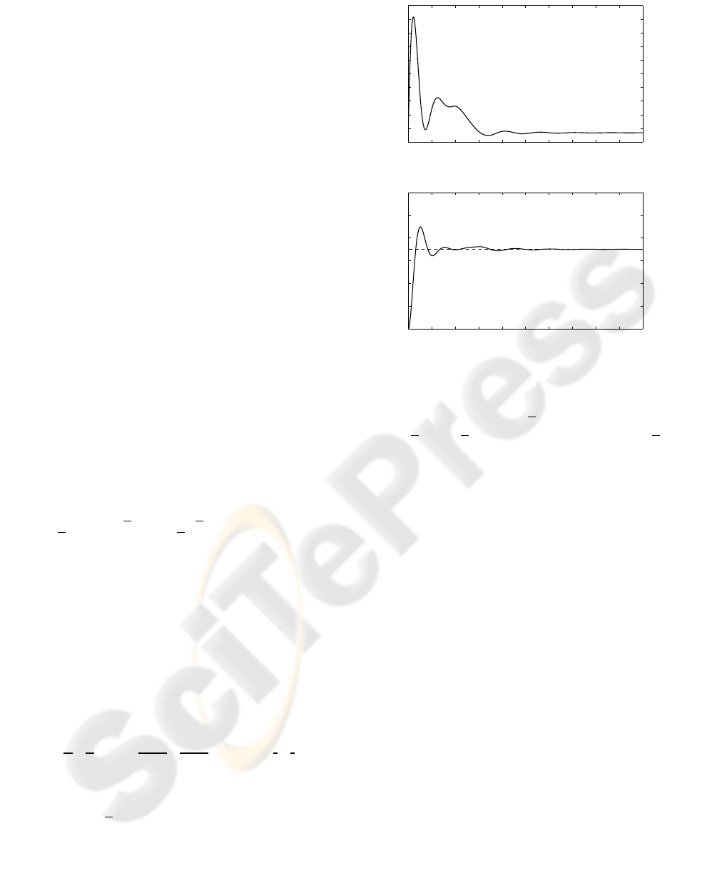
Input u
0 2 4 6 8 10 12 14 16 18 20
0
2
4
6
8
10
12
Output y
Time (s)
− − − reference
Figure 2: Simulation results of nominal control system.
form ˙x
s
= (α
1
A
s
(
¯
ρ) +α
2
A
s
(ρ
))x
s
+ B
s
u, where α
1
=
(ρ(t) − ρ)/(
¯
ρ − ρ), and α
2
= (−ρ(t) +
¯
ρ)/(
¯
ρ − ρ).
Then the results of Theorem 1 are used to design the
controller to stabilize the closed loop system, and to
track the desired constant reference signal. Figure 2
shows that the controlled system output reaches the
desired set point with ”almost” perfect tracking.
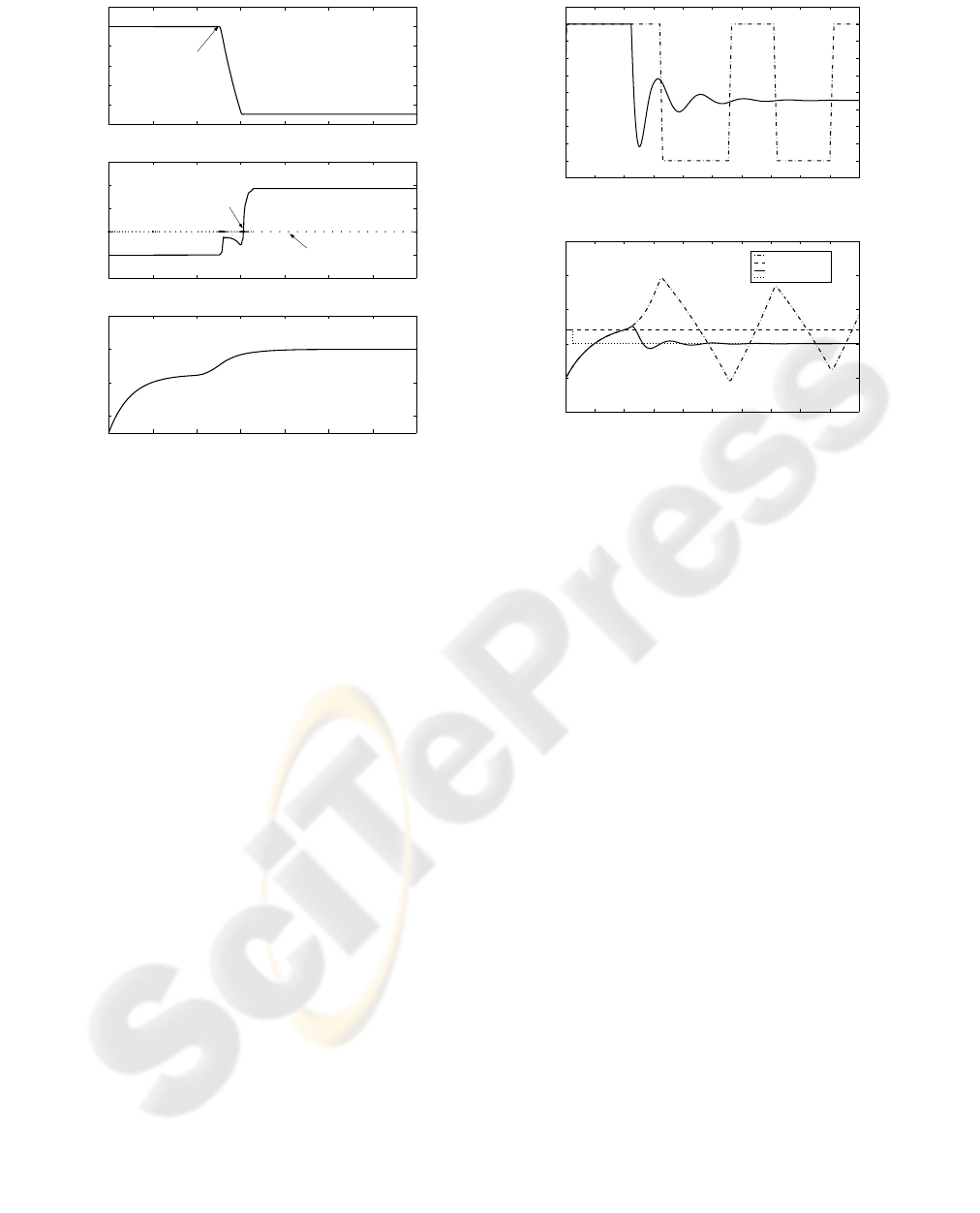
4.2 Fault Diagnosis
The proposed design of saturation fault diagnosis is
simulated for the LPV model (20). Figure 3 shows
the results of fault diagnostic system with the satura-
tion level of δ = 0.5. The fault is occurred at 5.00 sec
and detected at 6.12 sec using the threshold value of
0.05. The results of Theorem 2 are used to estimate
the saturation level. The learning rate Γ is chosen as
Γ = 10, and the filter pole is set to p = −60. Figure 3
shows that after the occurrence of the fault, the level
of the saturation fault is converged to the true value
within about 3 sec. The result indicates that the esti-
mation scheme provides an accurate estimation of the
saturation level within a reasonable time.
4.3 Fault Accommodation
Once the saturation level is estimated and sent to the
reconfiguration mechanism scheme. An appropriate
reconfiguration of the feed-forward gain and refer-
0 2 4 6 8 10 12 14
−0.25
−0.2
−0.15
−0.1
−0.05
0
0.05
Fault Indication (λ)
0 2 4 6 8 10 12 14
−0.05
0
0.05
0.1
0.15
0.2
Average Energy of λ
0 2 4 6 8 10 12 14
0
0.1
0.3
0.5
0.7
Estimation of Sat. Level
Time (s)
Fault occurrence
(5.00 sec)
Threshold = 0.05
Fault detection
(6.12 sec)
Figure 3: Simulation results of fault diagnostic scheme.
ence reshaping filter is triggered to accommodate the
fault. Figure 4 shows the simulation results of the
control system with and without fault accommoda-
tion for the case of 0.2 reduction in the saturation
limit. Without fault accommodation, the input sig-
nal reaches its limit and the output diverges from the
desired set point. With fault accommodation, on the
other hand, the input signal is reduced within its new
limit and the output tracks the desired set point.
5 CONCLUSION
Designing a FTC system for LPV systems subject to
actuator saturation fault is considered. The FTC sys-
tem consists of a nominal control, fault diagnostic,
and fault accommodation schemes in order to achieve
control objectives in the absence and presence of ac-
tuator saturation fault. Simulation results demonstrate
the effectiveness of the proposed FTC system.
REFERENCES
Apkarian, P. and Adams, R. J. (1998). Advanced gain-
scheduling techniques for uncertain systems. IEEE
Transaction on Control Systems Technology, 6:21–32.
Apkarian, P., Gahinet, P., and Becker, G. (1995). Self-
scheduled h
∞
control of linear parameter-varying sys-
tems: a design example. Automatica, 31:1251–1261.
Bara, G. I., Daafouz, J., Kratz, F., and Ragot, J. (2001).
Parameter-dependent state observer design for affine
0 2 4 6 8 10 12 14 16 18 20
−5
−4
−3
−2
−1
0
1
2
3
4
5
Input u
0 2 4 6 8 10 12 14 16 18 20
−5
0
5
10
15
20
Output y
Time (s)
Without fault accom.
Reference
With fault accom.
Modified reference
Figure 4: Simulation results with and without fault accom-
modation.
lpv systems. International Journal of Control,
74:1601–1611.
Blanke, M., Staroswiecki, M., and Wu, N. E. (2001). Con-
cepts and methods in fault-tolerant control. In proc.
American Control Conference.
Bodson, M. (1995). Emerging technologies in control engi-
neering. IEEE Control Systems Magazine, 15.
Gahinet, P., Apkarian, P., and Chilali, M. (1996). Affine
parameter-dependent lyapunov functions and real
parametric uncertainty. IEEE Transaction on Auto-
matic Control, 41:436–442.
Isermann, R., Schwarz, R., and Stolzl, S. (2002). Fault-
tolerant drive-by-wire systems. IEEE Control Systems
Magazine, 22.
Kose, I. E., Jabbari, F., and Schmitendorf, W. E. (1998).
A direct characterization of l2-gain controllers for lpv
systems. IEEE Transaction on Automatic Control,
43:1302–1307.
Patton, R. J. (1997). Fault-tolerant control systems: the
1997 situation. In SAFEROCESS’97, IFAC Symp.
Fault Detection, Supervision and Safety for Technical
Processes.
Polycarpou, M. M. and Helmicki, A. J. (1995). Automated
fault detection and accommodation: a learning sys-
tems approach. IEEE Transactions on Systems, Man
and Cybernetics, 25.
Rauch, H. E. (1994). Intelligent fault diagnosis and control
reconfiguration. IEEE Control Systems Magazine, 14.
Stengel, R. F. (1991). Intelligent failure-tolerant control
systems. IEEE Control Systems Magazine, 11.
Tuan, H. D. and Apkarian, P. (2002). Monotonic relaxations
for robust control: new characterizations.
