
A MODIFIED IMPULSE CONTROLLER FOR IMPROVED
ACCURACY OF ROBOTS WITH FRICTION
Stephen van Duin, Christopher D. Cook, Zheng Li and Gursel Alici
Faculty of Engineering, University of Wollongong, Northfields Avenue, Gwynnville, Australia
Keywords: Impulsive control, static friction, limit cycle, stick-slip, impulse shape, friction model, accuracy.
Abstract: This paper presents a modified
impulse controller to improve the steady state positioning of a SCARA robot
having characteristics of high non-linear friction. A hybrid control scheme consisting of a conventional PID
part and an impulsive part is used as a basis to the modified controller. The impulsive part uses short width
torque pulses to provide small impacts of force to overcome static fiction and move a robot manipulator
towards its reference position. It has been shown that this controller can greatly improve a robot’s accuracy.
However, the system in attempting to reach steady state will inevitably enter into a small limit cycle whose
amplitude of oscillation is related to the smallest usable impulse. It is shown in this paper that by modifying
the impulse controller to adjust the width of successive pulses, the limit cycle can be shifted up or down in
position so that the final steady state error can be even further reduced.
1 INTRODUCTION
Precision robot manufacturers continually strive to
increase the accuracy of their machinery in order to
remain competitive. The ability of a robot
manipulator to position its tool centre point to within
a very high accuracy, allows the robot to be used for
more precise tasks. For positioning of a tool centre
point, the mechanical axes of a robot will be
required to be precisely controlled around zero
velocity where friction is highly non-linear and
difficult to control.
Non-linear friction is naturally present in all
mechanism
s and can cause stick-slip during precise
positioning. In many instances, stick-slip has been
reduced or avoided by modifying the mechanical
properties of the system; however this approach may
not always be practical or cost effective.
Alternatively, advances in digital technology have
made it possible for the power electronics of
servomechanisms to be controlled with much greater
flexibility. By developing better controllers, the
unfavourable effects of non-linear friction may be
reduced or eliminated completely.
Impulse control has been successfully used for
accurate positioni
ng of servomechanisms with high
friction where conventional control schemes alone
have difficulty in approaching zero steady state
error. Static and Coulomb friction can cause a
conventional PID controller having integral action
(I), to overshoot and limit cycle around the reference
position. This is a particular problem near zero
velocities where friction is highly non linear and the
servomechanism is most likely to stick-slip. Despite
the above difficulties, PID controllers are still
widely used in manufacturing industries because of
their robustness to parameter uncertainty and
unknown disturbances.
Stick-slip can be reduced or eliminated by using
i
mpulsive control near or at zero velocities. The
impulsive controller is used to overcome static
friction by impacting the mechanism and moving it
by microscopic amounts. By combining the
impulsive controller and conventional controller
together, the PID part can be used to provide
stability when moving towards the reference
position while the impulse controller is used to
improve accuracy for the final positioning where the
error signal is small.
By applying a short impulse of sufficient force
p
lastic deformation occurs between the asperities of
mating surfaces resulting in permanent controlled
movement. If the initial pulse causes insufficient
movement, the impulsive controller produces
additional pulses until the position error is reduced
to a minimum.
165
van Duin S., D. Cook C., Li Z. and Alici G. (2007).
A MODIFIED IMPULSE CONTROLLER FOR IMPROVED ACCURACY OF ROBOTS WITH FRICTION.
In Proceedings of the Fourth International Conference on Informatics in Control, Automation and Robotics, pages 165-173
DOI: 10.5220/0001618901650173
Copyright
c
SciTePress
a)
b)
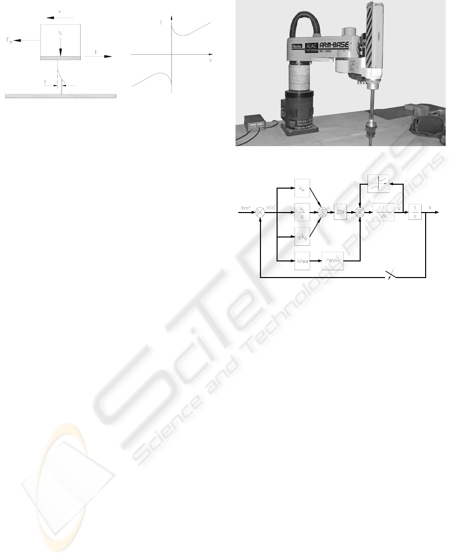
Figure 1: Bristle model; Figure a) shows the deflection of a
single bristle. Figure b) shows the resulting static friction
model for a single instance in time.
A number of investigators have devised
impulsive controllers which achieve precise motion
in the presence of friction by controlling the height
or width of a pulse. Yang and Tomizuka (Yang et al,
1988) applied a standard rectangular shaped pulse
whereby the height of the pulse is a force about 3 to
4 times greater than the static friction to guarantee
movement. The width of the pulse is adaptively
adjusted proportional to the error and is used to
control the amount of energy required to move the
mechanism towards the reference positioning.
Alternatively, Popovic (Popovic et al, 2000)
described a fuzzy logic pulse controller that
determines both the optimum pulse amplitude and
pulse width simultaneously using a set of
membership functions. Hojjat and Higuchi (Hojjat
et al, 1991) limited the pulse width to a fixed
duration of 1ms and vary the amplitude by applying
a force about 10 times the static friction. Rathbun et
al (Rathbun et al, 2004) identify that a flexible-body
plant can result in a position error limit cycle and
that this limit cycle can be eliminated by reducing
the gain using a piecewise-linear-gain pulse width
control law.
In a survey of friction controllers by Armstrong-
Hélouvry (Armstrong- Hélouvry et al, 1994), it is
commented that underlying the functioning of these
impulsive controllers is the requirement for the
mechanism to be in the stuck or stationary position
before subsequent impulses are applied. Thus,
previous impulse controllers required each small
impacting pulse to be followed by an open loop slide
ending in a complete stop.
Figure 2: The Hirata SCARA robot.
Figure 3: Block diagram of the experimental system
controller.
In this paper, a hybrid PID + Impulsive
controller is used to improve the precision of a
servomechanism under the presence of static and
Coulomb friction. The design and functioning of the
controller does not require the mechanism to come
to rest between subsequent pulses, making it suitable
for both point to point positioning and speed
regulation. The experimental results of this paper
show that the shape of the impulse can be optimised
to increase the overall precision of the controller. It
is shown that the smallest available movement of the
servomechanism can be significantly reduced
without modification to the mechanical plant.
2 MODELLING AND
EXPERIMENTAL SYSTEM
2.1 Friction Model
On a broad scale, the properties of friction are both
well understood and documented. Armstrong-
Hélouvry (Armstrong- Hélouvry et al, 1994) have
surveyed some of the collective understandings of
how friction can be modelled to include the
ICINCO 2007 - International Conference on Informatics in Control, Automation and Robotics
166

complexities of mating surfaces at a microscopic
level. Canudas de Wit (Canudas de Wit et al, 1995)
add to this contribution by presenting a new model
that more accurately captures the dynamic
phenomena of rising static friction (Rabinowicz,
1958), frictional lag (Rabinowicz, 1958), varying
break away force (Johannes et al, 1973),
(Richardson et al, 1976), dwell time (Kato et al,
1972), pre-sliding displacement (Dahl, 1968), (Dahl,
1977), (Johnson, 1987) and Stribeck effect (Olsson,
1996). The friction interface is thought of as a
contact between elastic bristles. When a tangential
force is applied, the bristles deflect like springs
which give rise to the friction force (Canudas de Wit
et al, 1995); see Figure 1(a). If the effective applied
force F
e
exceeds the bristles force, some of the
bristles will be made to slip and permanent plastic
movement occurs between each of the mating
surfaces. The set of equations governing the
dynamics of the bristles are given by (Olsson, 1996):
()
z
vg
v
v
dt
dz
−= (1)
() ()
()
(
2
0
1
s
vv
CsC
gv F F F e
σ
−
=+−
)
(2)
()
vF
dt
dz
vzF
v
++=
10
σσ
(3)
()
()
2
11
d
vv
ve
σσ
−
=
(4)
where v is the relative velocity between the two
surfaces and z is the average deflection of the
bristles.
σ
0
is the bristle stiffness and σ
1
is the bristle
damping. The term v
s
is used to introduce the
velocity at which the Stribeck effect begins while
the parameter v
d
determines the velocity interval
around zero for which the velocity damping is
active. Figure 1(b) shows the friction force as a
function of velocity. F
s
is the average static friction
while F
C
is the average Coulomb friction. For very
low velocities, the viscous friction F
v
is negligible
but is included for model completeness. F
s
, F
C
, and
F
v
are all estimated experimentally by subjecting a
real mechanical system to a series of steady state
torque responses. The parameters
σ
0,
σ
1,
v
s
and v
d
are
also determined by measuring the steady state
friction force when the velocity is held constant
(Canudas de Wit et al, 1995).
2.2 Experimental System
For these experiments, a Hirata ARi350 SCARA
(Selective Compliance Assembly Robot Arm) robot
was used. The Hirata robot has four axes named A,
B, Z and W. The main rotational axes are A-axis
(radius 350mm) and B-axis (radius 300mm) and
they control the end-effector motion in the
horizontal plane. The Z-axis moves the end-effector
in the vertical plane with a linear motion, while the
W-axis is a revolute joint and rotates the end effector
about the Z-axis. A photograph of the robot is
shown in Figure 2.
For these experiments, only the A and B axis of
the Hirata robot are controlled. Both the A and B
axes have a harmonic gearbox between the motor
and robot arm. Their gear ratios are respectively
100:1 and 80:1. All of the servomotors on the Hirata
robot are permanent magnet DC type and the A and
B axis motors are driven with Baldor® TSD series
DC servo drives. Each axis has characteristics of
high non-linear friction whose parameters are
obtained by direct measurement. For both axes, the
static friction is approximately 1.4 times the
Coulomb friction.
Matlab’s xPC target oriented server was used to
provide control to each of the servomotor drives. For
these experiments, each digital drive was used in
current control mode which in effect means the
output voltage from the 12-bit D/A converter gives a
torque command to the actuator’s power electronics.
The system controller was compiled and run using
Matlab’s real time xPC Simulink® block code. A
12-bit A/D converter was used to read the actuator’s
shaft encoder position signal.
2.3 PID + Impulse Hybrid Controller
Figure 3 shows the block diagram of a PID linear
controller + impulsive controller. This hybrid
controller has been suggested by Li (Li et al, 1998)
whereby the PID driving torque and impulsive
controller driving torque are summed together. It is
unnecessary to stop at the end of each sampling
period and so the controller can be used for both
position and speed control.
The controller can be divided into two parts; the
upper part is the continuous driving force for large
scale movement and control of external force
disturbances. The lower part is an additional
proportional controller k
pwm
with a pulse width
modulated sampled-data hold (PWMH), and is the
basis of the impulsive controller for the control of
stick-slip.
A MODIFIED IMPULSE CONTROLLER FOR IMPROVED ACCURACY OF ROBOTS WITH FRICTION
167
The system controller is sampled at 2 kHz. The
impulse itself is sampled and applied at one
twentieth of the overall sampling period (i.e. 100
Hz) to match the mechanical system dynamics.
Figure 4 shows a typical output of the hybrid
controller for one impulse sampling period
τ
s
. The
pulse with height f
p
is added to the PID output.
Because the PID controller is constantly active, the
F
o
r
ce
Δ
fp
PID
Output
τ
s
Figure 4: Friction controller output.
system has the ability to counteract random
disturbances applied to the servomechanism. The
continuous part of the controller is tuned to react to
large errors and high velocity, while the impulse part
is optimized for final positioning where stiction is
most prevalent.
For large errors, the impulse width approaches
the full sample period
τ
s
, and for very large errors, it
transforms into a continuous driving torque. When
this occurs, the combined control action of the PID
controller and the impulsive controller will be
continuous. Conversely, for small errors, the PID
output is too small to have any substantial effect on
the servomechanism dynamics.
The high impulse sampling rate, combined with a
small error, ensures that the integral (I) part of the
PID controller output has insufficient time to rise
and produce limit cycling. To counteract this loss of
driving torque, when the error is below a threshold,
the impulsive controller begins to segment into
individual pulses of varying width and becomes the
primary driving force. One way of achieving this is
to make the pulse width Δ determined by:
p
spwm
f
kek
τ
)(⋅
=Δ
if
|||)(|k
pwm p
fke
≤
⋅
s
τ
=Δ
otherwise (6)
In (6)
(
()
pp
)
f
fsignek=⋅
(7)
where e(k) is the error input to the controller, |f
p
|
is a fixed pulse height greater than the highest static
friction and
τ
s
is the overall sampling period. For
the experimental results of this paper, the impulsive
sampling period
τ
s
was 10ms and the pulse width
could be incrementally varied by 1ms intervals. The
pulse width gain k
pwm
, is experimentally determined
by matching the mechanism’s observed
displacement d to the calculated pulse width t
p
using
the equation of motion:
2
()
2
pp C
p
C
ff f
dt
mf
−
=
, f
p
> 0 (8)
The gain is iteratively adjusted until the net
displacement for each incremental pulse width is as
small as practical.
2.4 Minimum Pulse Width
The precision of the system is governed by the
smallest incremental movement which will be
produced from the smallest usable width pulse.
Because the shape of the pulse is affected by the
system’s electrical circuit response, a practical limit
is placed on the amplitude of the pulse over very
short durations and this restricts the amount of
energy that can be contained within a very thin
pulse. Consequently, there exists a minimum pulse
width that is necessary to overcome the static
friction and guarantee plastic movement.
For the Hirata robot, the minimum pulse width
guaranteeing plastic displacement was determined to
be 2ms and therefore the pulse width is adjusted
between 2 and 10ms. Any pulse smaller than 2ms
results in elastic movement of the mating surfaces in
the form of pre-sliding displacement. In this regime,
short impulses can produce unpredictable
displacement or even no displacement at all. In some
cases, the mechanism will spring back greater than
the forward displacement resulting in a larger error.
Figure 5 shows the displacement of the experimental
system of five consecutive positive impulses
followed by five negative impulses. The experiment
compares impulses of width 2ms and 1.5ms. For
impulses of 2ms, the displacement is represented by
the consistent staircase movement. For a width of
1.5ms, the displacement is unpredictable with
ICINCO 2007 - International Conference on Informatics in Control, Automation and Robotics
168
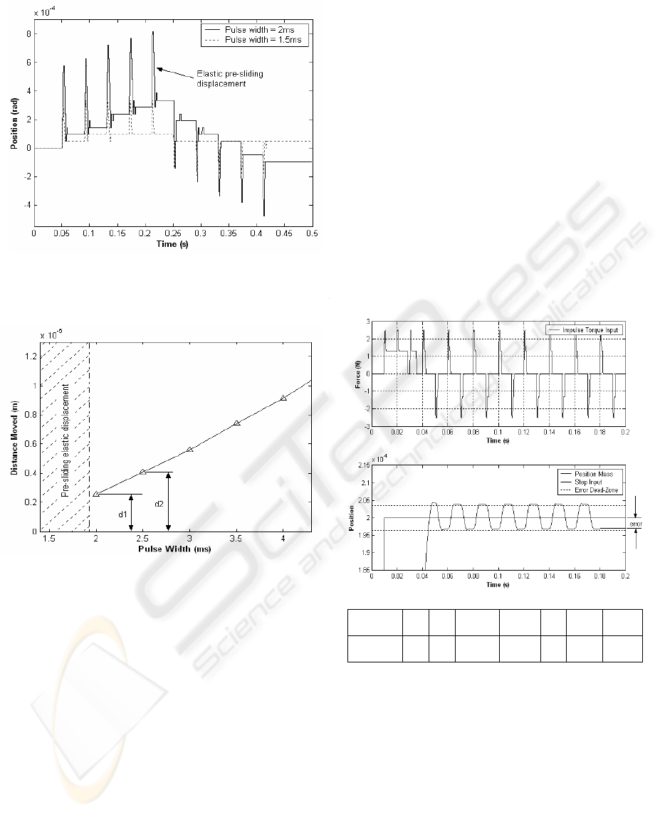
Figure 5: Experimentally measured displacement for both
positive and negative impulses using successive pulse
widths 1.5ms and 2ms.
Figure 6: Simulated displacements as a function of pulse
width.
mostly elastic pre-sliding movement which results in
zero net displacement.
Wu et al (Wu et al, 2004) use the pre-sliding
displacement as a means to increase the precision of
the controller by switching the impulse controller off
and using a continuous ramped driving torque to
hold the system in the desired position. The torque is
maintained even after the machine is at rest. This is
difficult in practice as pre-sliding movement must be
carefully controlled in the presence of varying static
friction so that inadvertent breakaway followed by
limit cycling is avoided.
3 LIMIT CYCLE OFFSET
3.1 Motivation
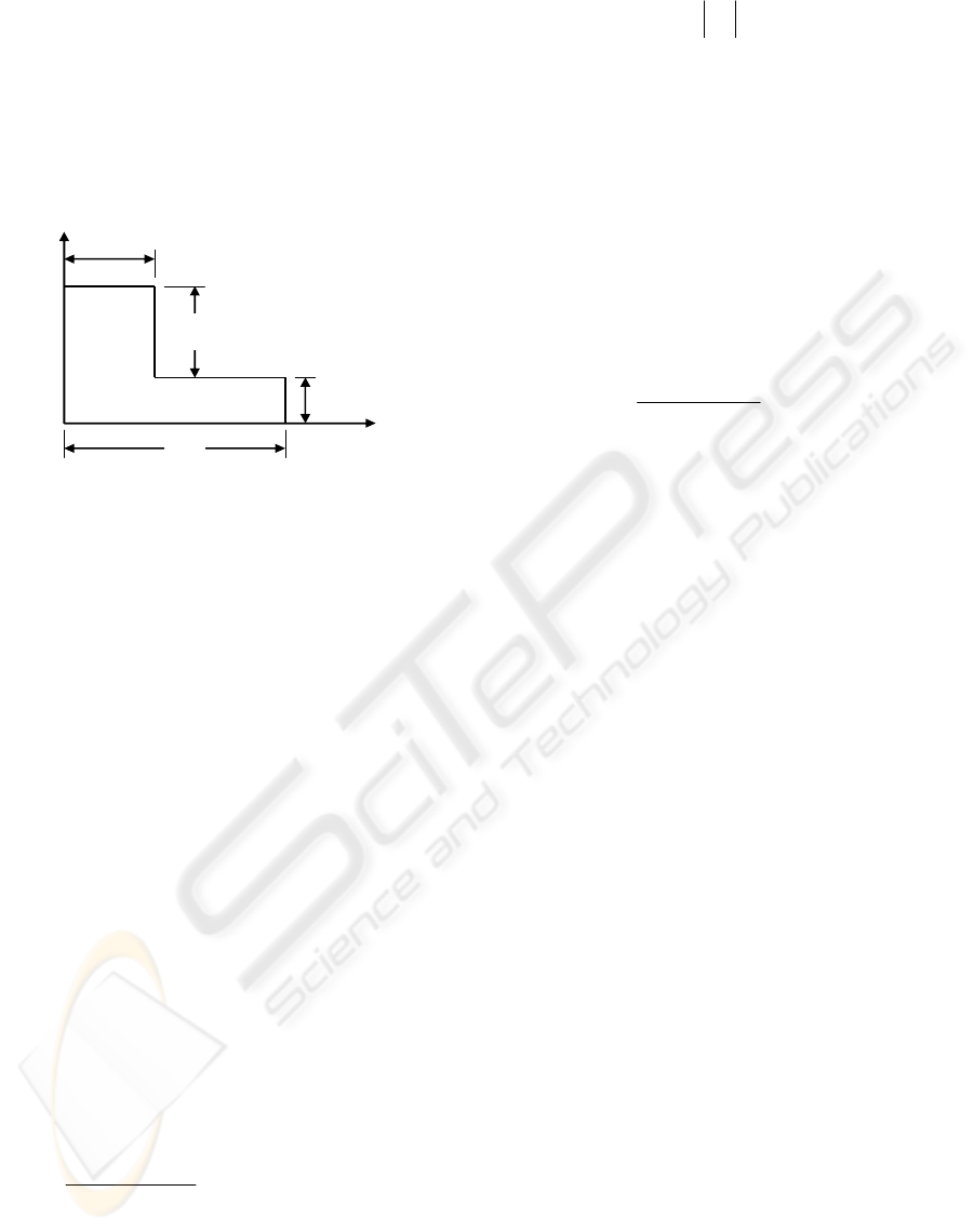
Figure 6 shows the simulated displacements of
varying pulse widths which have been labelled d1,
d2, d3…dn respectively, where d1 is the minimum
pulse width which will generate non elastic
movement and defines the system’s resolution.
Using the variable pulse width PID + impulse
controller for a position pointing task, the torque will
incrementally move the mechanism towards the
reference set point in an attempt to reach steady
state. Around the set point, the system will
inevitably begin to limit cycle when the error e(k) is
approximately the same magnitude as the system
resolution (the displacement for the minimum pulse
width d1).
Figure 7: Simulation of the impulse controller limit
cycling around a position reference set-point where the
final torque output is a pulse with a minimum width and
the mean peak to peak oscillation is d1. The friction
parameters used for the simulation are also given in the
accompanying table.
For the limit cycle to be extinguished, the
controller must be disabled. As an example, the limit
cycle in Figure 7 is extinguished by disabling the
impulse controller at t=0.18s, and in this case, the
resulting error is approximately half the
displacement of the minimum pulse width d1.
Parameter F
s
F
C
σ
0
σ
1
F
v
v
s
v
d
Value 2 1 4.5*10
5
12,000 0.4 0.001 0.0004
A MODIFIED IMPULSE CONTROLLER FOR IMPROVED ACCURACY OF ROBOTS WITH FRICTION
169
Limit cycling will occur for all general
servomechanisms using a torque pulse because
every practical system inherently has a minimum
pulse width that defines the system’s resolution.
Figure 7 simulates a typical limit cycle with a peak
to peak oscillation equal to the displacement of the
minimum pulse width d1.
One way to automatically extinguish the limit
cycle is to include a dead-zone that disables the
controller output when the error is between an upper
and lower bound of the reference point (see Figure
7). The final error is then dependent on the amount
of offset the limit cycle has in relation to the
reference point. Figure 7 shows a unique case where
the ± amplitude of the limit cycle is almost evenly
distributed either side of the reference set point; i.e.
the centre line of the oscillation lies along the
reference set point. In this instance, disabling the
controller would create an error e(k) equal to
approximately
d1
2
. This however, would vary in
practice and the centreline is likely to be offset by
some arbitrary amount. The maximum precision of
the system will therefore be between d1 and zero.
reference
position
d2 - d1
new
error
Time
Position
Figure 8: Conceptual example of reducing the steady state
error using ‘Limit Cycle Offset’ with the limit cycle shifted
up by d2-d1 and the new error that is guaranteed to fall
within the dead-zone.
3.2 Limit Cycle Offset Function
By controlling the offset of the limit cycle
centreline, it is possible to guarantee that the final
error lies within the dead-zone, and therefore to
increase the precision of the system. As a conceptual
example, Figure 8 shows a system limit cycling
either side of the reference point by the minimum
displacement d1. By applying the next smallest
pulse d2, then followed by the smallest pulse d1, the
limit cycle can be shifted by d2 – d1. The effect is
that the peak to peak centreline of the oscillation has
now been shifted away from the reference point.
However, at least one of the peaks of the
oscillation has been shifted closer to the set point. If
the controller is disabled when the mechanism is
closest to the reference set point, a new reduced
error is created. For this to be realised, the
incremental difference in displacement between
successively increasing pulses must be less than the
displacement from the minimum pulse width; for
example d2 – d1 < d1.
3.3 Modified Controller Design
For the limit cycle to be offset at the correct time,
the impulse controller must have a set of additional
control conditions which identify that a limit cycle
has been initiated with the minimum width pulse.
The controller then readjusts itself accordingly using
a ‘switching bound’ and finally disables itself when
within a new specified error ‘dead-zone’. One way
to achieve this is to adjust the pulse width so that it
is increased by one increment when satisfying the
following conditions:
if switching bound > |e(k)| ≥ dead-zone
then
()
1
pwm s
p
kek
f
τ
⋅
Δ
=+
otherwise
()
p
wm s
p
kek
f
τ
⋅
Δ=
(9)
where the switching bound is given by:
d1
|switching bound| <
2
(10)
and the dead-zone is given by:
(d2 - d1)
dead-zone =
2
(11)
The steady state error e(k) becomes:
steady state
deadzone
e(k)
2
≤
(12)
ICINCO 2007 - International Conference on Informatics in Control, Automation and Robotics
170
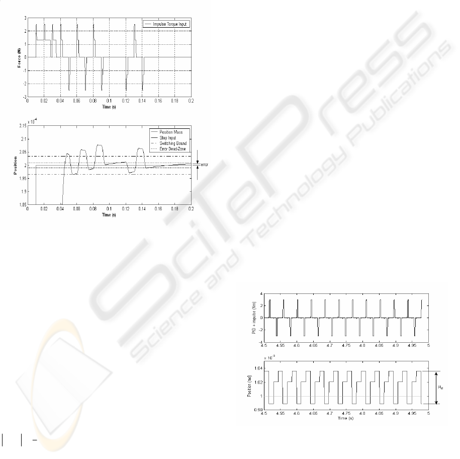
3.4 Simulation of the Limit Cycle
Offset Function
To demonstrate the limit cycle offset function, the
modified controller is simulated using a simple unit
mass with the ‘new’ friction model using Eqs. 1 to 4.
A simulated step response is shown in Figure 9
to demonstrate how the modified controller works.
Here the mechanism moves towards the reference
set point and begins limit cycling. Because at least
Figure 9: Simulation of the limit cycle offset function
used with the PID + impulse controller.
one of the peaks of the limit cycle immediately lies
within the switching bound, the controller shifts the
peak to peak oscillation by d2 - d1 by applying the
next smallest pulse, and then followed by the
smallest pulse. In this example, the first shift is
insufficient to move either peak into the set dead-
zone so the controller follows with a second shift. At
time 0.1 seconds, the controller is disabled;
however, the elastic nature of the friction model
causes the mechanism’s position to move out of the
dead-zone. As a result, the controller is reactivated
(time 0.12s) and the controller follows with a third
shift. In this instance, the mechanism reaches steady
state at t=0.2s, and the final error is
1
2
( ) (dead zone)ek ≤⋅
which in this case is ± 1e-6
radians. A final analysis of the result shows that the
new controller has reduced the error by an amount
significantly more than a standard impulse
controller. This reduction correlates directly to the
improvement in the system’s accuracy by a factor of
4.
4 EXPERIMENTAL
4.1 Position Pointing
This section evaluates the limit cycle offset function
using the experimental Hirata robot having position
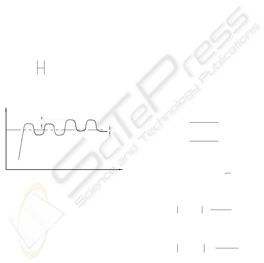
dependent variables. Figure 10 shows a steady state
limit cycle for a position pointing step response of
0.001 radians using a PID + impulse hybrid
controller. The mean peak to peak displacement of
the smallest non-elastic part of the limit cycle is μ
d
.
The experiment was repeated using the limit
cycle offset function with the same position step
reference of 0.001 radians. Figure 11 shows a
sample experiment and in this example, the limit
cycle offset function is activated at t=0.9s. At this
time, the amplitude of the non elastic part of the
limit cycle is identified as lying between the
switching bounds. The switching bounds and dead-
zone are set according to the methodology given
earlier. Once the offset function is activated, the
controller adjusts itself by forcing the proceeding
pulse to be one increment wider before returning to
the smallest pulse width. This results in the limit
cycle being shifted down into the dead-zone region
where the impulse controller is automatically
disabled at t=0.95s. At this time, the final error is
guaranteed to fall within the error dead zone which
can be seen from Fig 11 to be in the vicinity of ±1e-
4 radians.
Figure 10: Steady state limit cycle for the PID + impulse
hybrid controller when applying a unit step input to the
Hirata robot. The mean peak to peak displacement μ
d
is
the non-elastic part of limit cycle.
A MODIFIED IMPULSE CONTROLLER FOR IMPROVED ACCURACY OF ROBOTS WITH FRICTION
171
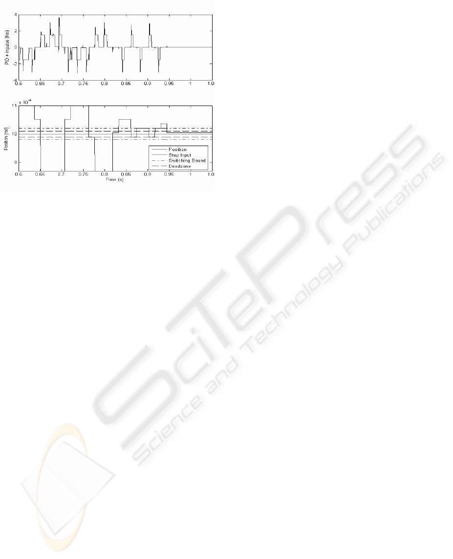
Figure 11: Using the ‘Limit Cycle Offset’ function to
reduce the final steady state error of the Hirata robot.
4.2 Discussion of Results
This set of results demonstrates the Limit Cycle
Offset function can be successfully applied to a
commercial robot manipulator having characteristics
of high non-linear friction. The results show that the
unmodified controller will cause the robot to limit
cycle near steady state position and that the peak to
peak displacement is equal to the displacement of
the smallest usable width pulse.
By using the Limit Cycle Offset function, the
limit cycle can be detected and the pulse width
adjusted so that at least one of the peaks of the limit
cycle is moved towards the reference set point.
Finally, the results show that the controller
recognises the limit cycle as being shifted into a
defined error dead-zone whereby the controller is
disabled. The steady state error is therefore
guaranteed to fall within a defined region so that the
steady state error is reduced. For the SCARA robot,
the improvement in accuracy demonstrated was
1.1e-4 radians in comparison to 4.5e-4 radians
achieved without the limit cycle offset.
5 CONCLUSION
Advances in digital control have allowed the power
electronics of servo amplifiers to be manipulated in
a way that will improve a servomechanism precision
without modification to the mechanical plant. This is
particularly useful for systems having highly non-
linear friction where conventional control schemes
alone under perform. A previously developed hybrid
PID + Impulse controller which does not require the
mechanism to come to a complete stop between
pulses has been modified to further improve
accuracy. This modification shifts the limit cycling
into a different position to provide substantial
additional improvement in the mechanism’s position
accuracy. This improvement has been demonstrated
both in simulations and in experimental results on a
SCARA robot arm. The mechanism does not have to
come to a complete stop between pulses, and no
mechanical modification has to be made to the robot.
REFERENCES
Armstrong-Hélouvry, B., 1991, “Control of Machines with
Friction” Kluwer Academic Publishers, 1991, Norwell
MA.
Armstrong-Hélouvry, B., Dupont, P., and Canudas de
Wit, C., 1994, “A survey of models, analysis tools and
compensation methods for the control of machines
with friction” Automatica, vol. 30(7), pp. 1083-1138.
Canudas de Wit, C., Olsson, H., Åström, K. J., 1995 ”A
new model for control of systems with friction” IEEE
Tansactions on Automatic Control, vol. 40 (3), pp.
419-425.
Dahl, P., 1968, “A solid friction model” Aerospace Corp.,
El Segundo, CA, Tech. Rep. TOR-0158(3107-18)-1.
Dahl, P, 1977, “Measurement of solid friction parameters
of ball bearings” Proc. of 6
th
annual Symp. on
Incremental Motion, Control Systems and Devices,
University of Illinois, ILO.
Hojjat, Y., and Higuchi, T., 1991 “Application of
electromagnetic impulsive force to precise
positioning” Int J. Japan Soc. Precision Engineering,
vol. 25 (1), pp. 39-44.
Johannes, V. I.., Green, M.A., and Brockley,C.A., 1973,
“The role of the rate of application of the tangential
force in determining the static friction coefficient”,
Wear, vol. 24, pp. 381-385.
Johnson, K.L., 1987, “Contact Mechanics” Cambridge
University Press, Cambridge.
Kato, S., Yamaguchi, K. and Matsubayashi, T., 1972,
“Some considerations of characteristics of static
friction of machine tool slideway” J. o Lubrication
Technology, vol. 94 (3), pp. 234-247.
Li, Z, and Cook, C.D., 1998, ”A PID controller for
Machines with Friction” Proc. Pacific Conference on
Manufacturing, Brisbane, Australia, 18-20
August,
1998, pp. 401-406.
Olsson, H., 1996, “Control Systems with Friction”
Department of Automatic Control, Lund University,
pp.46-48.
Popovic, M.R., Gorinevsky, D.M., Goldenberg, A.A.,
2000, “High precision positioning of a mechanism
with non linear friction using a fuzzy logic pulse
ICINCO 2007 - International Conference on Informatics in Control, Automation and Robotics
172

controller” IEEE Transactions on Control Systems
Technology, vol. 8 (1) pp. 151-158.
Rabinowicz, E., 1958, “The intrinsic variables affecting
the stick-slip process,” Proc. Physical Society of
London, vol. 71 (4), pp.668-675.
Rathbun, D,. Berg, M. C., Buffinton, K. W., 2004,
“Piecewise-Linear-Gain Pulse Width Control for
Precise Positioning of Structurally Flexible Systems
Subject to Stiction and Coulomb Friction”, ASME J
.of Dynamic Systems, Measurement and Control,
vol. 126, pp. 139-126.
Richardson, R. S. H., and Nolle, H., 1976, “Surface
friction under time dependant loads” Wear, vol. 37
(1), pp.87-101.
Wu, R,. Tung, P., 2004, “Fast Positioning Control for
Systems with Stick-Slip Friction”, ASME J .of
Dynamic Systems, Measurement and Control, vol.
126, pp. 614-627.
Yang, S., Tomizuka, M., 1988, “Adaptive pulse width
control for precise positioning under the influence of
stiction and Coulomb friction” ASME J .of Dynamic
Systems, Measurement and Control, vol. 110 (3), pp.
221-227.
A MODIFIED IMPULSE CONTROLLER FOR IMPROVED ACCURACY OF ROBOTS WITH FRICTION
173
