EXTENSION OF THE GENERALIZED IMAGE RECTIFICATION
Catching the Infinity Cases
Klaus H
¨
aming and Gabriele Peters
LSVII, University of Dortmund, Otto-Hahn-Str. 16, D-44227 Dortmund, Germany
Keywords:
Stereo vision, epipolar geometry, rectification, image processing, object acquisition.
Abstract:
This paper addresses the topic of image rectification, a widely used technique in 3D-reconstruction and stereo
vision. The most popular algorithm uses a projective transformation to map the epipoles of the images to infin-
ity. This algorithm fails whenever an epipole lies inside an image. To overcome this drawback, a rectification
scheme known as polar rectification can be used. This, however, fails whenever an epipole lies at infinity.
For autonomous systems exploring their environment, it can happen that successive camera positions con-
stitute cases where we have an image pair with one epipole at infinity and the other inside an image. So
neither of the previous algorithms can be applied directly. We present an extension to the polar rectification
scheme. This extension allows the rectification of image pairs whose epipoles lie even at such difficult posi-
tions. Additionally, we discuss the necessary computation of the orientation of the epipolar geometry in terms
of the fundamental matrix directly, avoiding the computation of a line homography as in the original polar
rectification process.
1 INTRODUCTION
A common problem in all stereo vision tasks is the
correspondence problem. To simplify this search for
image structures representing the same world struc-
ture, images are usually rectified. The result is a pair
of images where corresponding points lie on the same
horizontal line, this way limiting the search region.
How this process is carried out in a given case
depends on the camera geometry. The epipoles are
points in the image plane induced by this geometry.
These points are the images of the camera centers,
i.e., the first epipole is the projection of the second
camera center onto the fist image plane and the sec-
ond epipole is the same for the first camera center. In
the original, non-rectified images, the corresponding
lines mentioned above all meet at the epipoles. So,
epipoles and their position play an important role in
image rectification.
In most stereo vision tasks the camera centers
have a distance of a few centimeters and the cameras
are pointing to a common point in front of them. In
those cases the epipoles neither lie inside an image
nor at infinity. This makes things easy and the tradi-
tional way of rectification through image homography
as described in popular textbooks such as (Hartley and
Zisserman, 2004) might be applied.
As our interest lies in object recognition and ob-
ject learning, including autonomous movements of
a camera guiding system (Peters, 2006), successive
camera positions are more or less unpredictable. This
means those special cases mentioned above can even
occur in combination, as shown in Figure 1.
For epipoles inside the image boundaries, the ap-
proach of polar rectification exists (Pollefeys et al.,
1999). Inside an image, the epipole divides each
epipolar line into two half-lines, thus limiting the
search region not only to epipolar lines, but to epipo-
lar half-lines. To exploit this advantage, the epipolar
geometry has to be oriented. In Pollefeys’ approach,
the orientation is carried out using a line homogra-
phy computed from the fundamental matrix or from
the camera projection matrices. Our approach uses
the fundamental matrix directly. This is described in
section 2.
The process of resampling the images to produce
275
Häming K. and Peters G. (2007).
EXTENSION OF THE GENERALIZED IMAGE RECTIFICATION - Catching the Infinity Cases.
In Proceedings of the Fourth International Conference on Informatics in Control, Automation and Robotics, pages 275-279
DOI: 10.5220/0001620802750279
Copyright
c
 SciTePress

Cam 1
Cam 2
a
b
c
2nd epipole
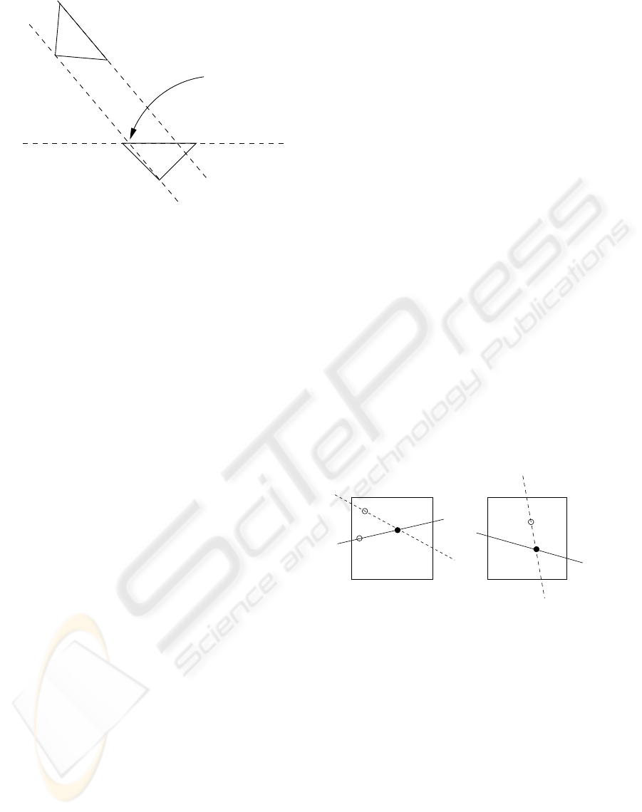
Figure 1: A difficult camera constellation for image recti-
fication. Line b connects both camera centers. The second
epipole lies at the position, where this line meets the image
plane a of “Cam 2”. In this case, this is inside the second
image. On the other hand, the first epipole lies at the posi-
tion where b meets c, the image plane of “Cam 1”. This is,
however, at infinity.
a rectified image pair is the topic of Section 3. First,
in Section 3.1, the procedure for epipoles at a finite
position will be reviewed shortly, then, in Section 3.2,
our extension for the case of infinity is presented.
As two rectification techniques already exist—on
the one hand polar rectification, which can handle
epipoles inside the image and on the other hand rec-
tification through image homography, which easily
handles epipoles at infinity—one can argue it may
be sufficient to switch to the appropriate one for the
given case. This will, unfortunately, not cover the
case in which one epipole lies inside and the other at
infinity. This case can easily occur as already shown
in Figure 1. To solve this problem, our extension of
the polar rectification method will now be discussed.
2 ORIENTATION
The polar rectification samples the epipolar lines one
by one and puts them one after another into a new im-
age. If the epipole lies inside the image, it will divide
the epipolar lines into two half-lines. That means, we
do not only have to match the correct epipolar lines
to each other, but the correct half of them. Otherwise
we have to search the whole epipolar line where half
the effort would suffice. Now the question is how to
tell which halfs belong to each other. To solve this,
we first have to orient the epipolar geometry. Un-
like Pollefeys in (Pollefeys et al., 1999) we do not
compute the line homography but use the fundamen-
tal matrix directly.
The fundamental matrix, denoted by F, describes
the relationship between two images and their cam-
eras known as the epipolar geometry. Let x
′
be a point
in the first view, then
l
′′
= Fx
′
(1)
is the the line in the second view on which any corre-
sponding point of x
′
must lie. Similarly, there exists a
relation
l
′
= F
T
x
′′
(2)
between a point x
′′
in the second view and a line l
′
in the first view. These lines are 3-vectors of the co-
efficients of the equation of an implicit line in two
dimensions:
l
′
0
∗ x+ l
′
1
∗ y+ l
′
2
= 0 (3)
Therefore each line divides the plane into a positive
and a negative region. This can be used to orient the
epipolar geometry.
Usually “orient the epipolar geometry” means to
ensure that every world point seen by one of the cam-
eras lies in front of this very camera. The usefulness
of oriented epipolar geometry for computer vision
was first described by St
´
ephane Laveau in (Laveau
and Faugeras, 1996).
However, what we like to know is on which side
of their epipolar lines with respect to the epipoles lie
two corresponding points.
p’’
e’
e’’
p’
k’
k’’=Fx’
x’
Figure 2: A visualization of the orientation process. The
symbols correspond to those in Equation 4 and 5. Essen-
tially, after orientation, the sign of the fundamental matrix
F is modified in such a way that the regions in which p
′
and
p
′′
lie have the same sign with respect to the lines k
′
and k
′′
.
To answer our question, we use equations 1 and 2
and a pair of points initially known to constitute a cor-
respondence. As in Figure 2, the point pair is denoted
by p
′
and p
′′
for the point in the first and second view,
respectively. We use an auxiliary line
k
′
= x
′
× e
′
(4)
where x
′
is an arbitrary point (with the exception that
it must not lie on the line p
′
× e
′
) and e
′
is the first
epipole. Then we choose the sign s in such a way that
sign (k
′
p
′
) = s· sign ((Fx
′
)p
′′
) (5)
ICINCO 2007 - International Conference on Informatics in Control, Automation and Robotics
276

where Fx
′
is k
′′
, the line in the second image corre-
sponding to k
′
. Having s computed, we can orient our
fundamental matrix
F
o
= sF (6)
Having the oriented fundamental matrix F
o
, the
correct half-line is easily determined. Suppose there
is a point q
′
in the first image and the appropriate line
in the second image is t
′′
= Fq
′
. For each candidate
q
′′
on the correct half-line of t
′′
sign ((e
′
× p
′
) · q
′
) = sign ((F
o
p
′
) · q
′′
) (7)
must hold true. Thus, we have limited the search re-
gion from epipolar lines to epipolar half-lines.
When using polar rectification, make sure all
quantities used in equation 7 retain their sign through-
out the process. Otherwise the result will be disap-
pointing even if F is oriented first.
3 RECTIFICATION
In this section, we will first review the re-sampling
process via polar rectification as described by Polle-
feys. Then, we will introduce our proposed extension
for epipoles at infinity.
3.1 Resampling the Image
The main idea is to sample the image one epipolar line
after another. This leads to the question about an ap-
propriate step size between successive epipolar lines.
The main criterion is to avoid a too coarse sampling,
meaning a loss of information contained in the image.
Figure 3 visualizes how to determine a good dis-
tance between successive epipolar lines. It shows two
congruent right-angled triangles defined by the point
triplets abc and a
′
b
′
c
′
. Both have the point b = b
′
in
common. Now, the goal is to ensure that the distance
|c
′
a
′
| is at least one pixel.
Exploiting the observed congruency, the distance
|c
′
b
′
| along the image border can be computed as the
ratio
|c
′
b
′
| =
|bc|
|ac|
(8)
The same is done in the second image. The result-
ing point is transferred into the first image by ap-
plying equation 2 and intersecting the resulting line
with the image border. Point b
′′
denotes the result. If
|c
′
b
′
| < |c
′
b
′′
|, the step size of the first image is used,
otherwise the step size of the second image is used.
Obviously, if one of the epipoles approaches infin-
ity, this procedure will fail because in equation 8 both
numerator and denominator also approach infinity.
a
c’
b
b’=b
a’
c=epipole
transferred
line
b’’
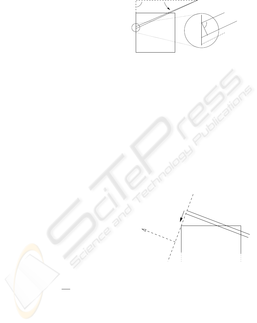
Figure 3: Resampling of an image using polar rectification.
The two congruent right-angled triangles abc and a
′
b
′
c
′
are
shown. The line computed from the step size in the second
image is depicted as “transferred line”. Its intersection with
the image border is b
′′
.
3.2 Resampling an Image with its
Epipole at Infinity
When the epipole approaches infinity, the left side of
equation 8 approximates one, which is our step size
for this case. The third co-ordinate of the epipole
equals or gets close to zero and the first two coordi-
nates form a 2D-vector pointing to the epipole. This
allows us to compute the perpendicular direction and
sample the image along this direction in parallel lines
using unit steps. This is shown in Figure 4. Of course,
this unit step again is compared to the step size of the
other image to avoid loss of information.
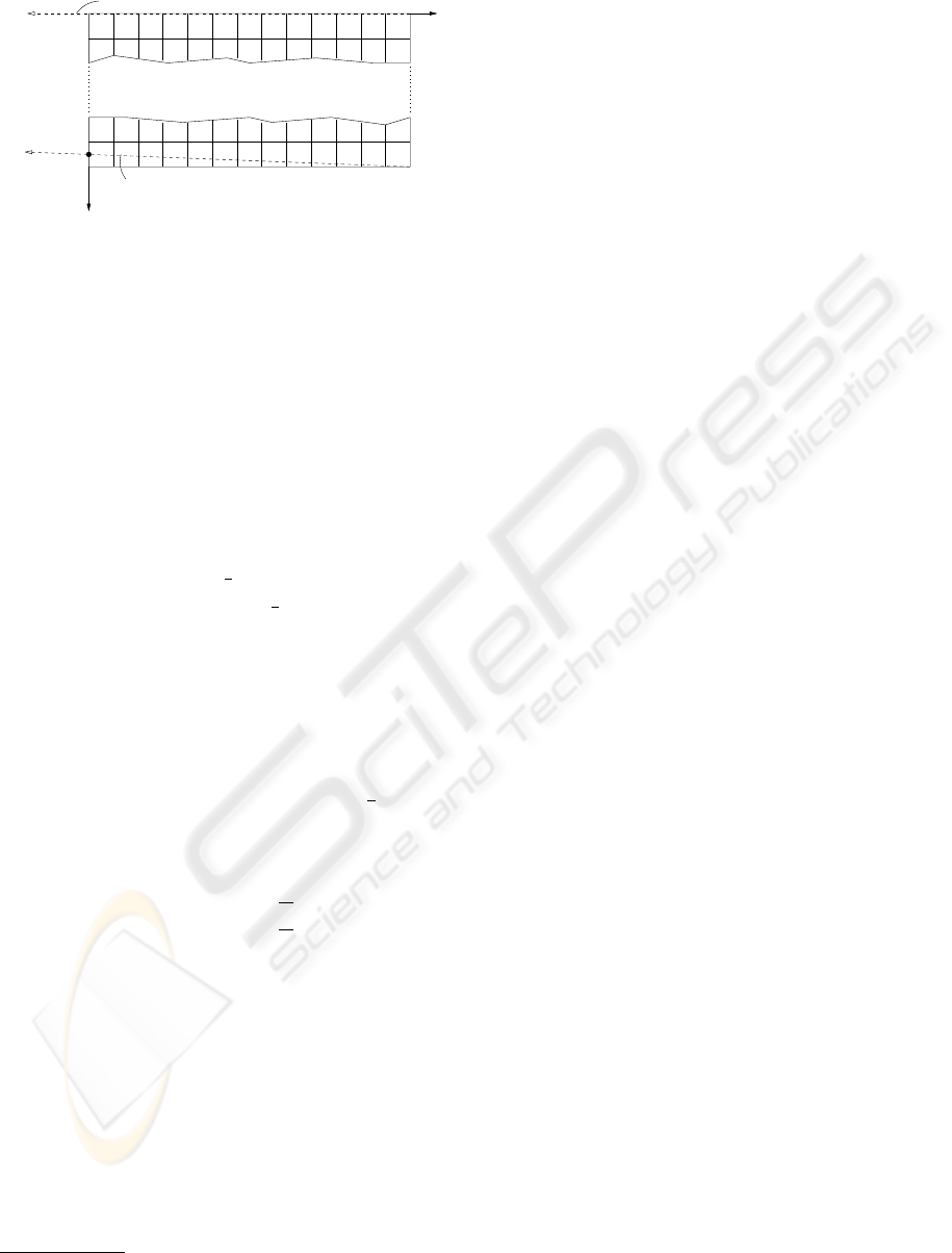
to epipole
Figure 4: If the epipole lies at infinity, the sampling can
easily be done scanning the image line by line perpendicular
to the direction of the epipole. The line distances are at most
one pixel.
To decide whether an epipole lies at infinity or not,
a threshold on the distance of the epipole to the image
jumps out as the natural parameter of choice. This
distance threshold is now denoted by d, the epipole
by e. Figure 5 shows how to compute a satisfying
value of d. The width of the image is w, the height is
h.
To simplify, we assume e = (e
0
, 0, 1)
T
, meaning
f = (0, 1, 0)
T
is an epipolar line. Thus, we can com-
EXTENSION OF THE GENERALIZED IMAGE RECTIFICATION - Catching the Infinity Cases
277

to epipole
to epipole
a
g
x
y
f
Figure 5: Finding a distance threshold d. A usable value
is computed as the horizontal distance of the epipole to the
image. The epipole in turn lies at the intersection of the
epipolar lines g and h.
pute |e
0
| as an appropriate value for d.
In our simplified consideration, we look at the
epipolar lines f and g, the latter intersecting the lower
right corner. The epipole may be assumed to lie
near infinity whenever these epipolar lines run par-
allel “enough”. g also intersects the left image border
in a point denoted by a. The distance of point a to the
lower left image corner can be used to compute the
value of e
0
.
Choosing a distance of
1
2
pixel from a to the lower
left corner, we get a = (0,h −
1
2
, 1)
T
. Because the
left image border is (1, 0, 0)
T
and g = (e×(w, h, 1)
T
),
a can also be computed as a = (1, 0, 0)
T
× (e ×
(w, h, 1)
T
). This yields e
0
= w− 2wh.
For an image with w = h = 1000, the epipole has
an x-coordinate of -1 999 000. For such an image
a distance threshold of more than 2 000 000 would
therefore be sufficient.
Once d is computed (or chosen), let ε = |
1
d
|. Then,
a usable rule to decide when to switch to sampling
with parallel lines looks like:
epipole
is at
infinity
⇔
(|e
2
| < ε)
OR
(|e
0
| > 0 AND (|
e
2
e
0
| < ε))
OR
(|e
1
| > 0 AND (|
e
2
e
1
| < ε))
(9)
It is advantageous to first compute the point pairs
on the image borders where in one of the images a
corner is met during rectification. Between two con-
secutive pairs, the whole process is merely a simple
loop of repeatedly determining the optimum step size
and sampling the images.
4 RESULTS
We examine our method proposed in section 3 with
two stereo pair examples shown in Figures 6 and 7
1
.
1
They show the freely available VRML model ”Al”
from different camera positions.
For both examples the rectified images are shown be-
low the original images. It can easily be recognized
that corresponding features now lie on the same line
which is, after all, what rectification is all about.
The initial point correspondence needed to orient
the epipolar geometry was not obtained through fea-
ture matching, but by intersecting the known view-
ing pyramids of the cameras and choosing the closest
point in a decent distance to both camera centers.
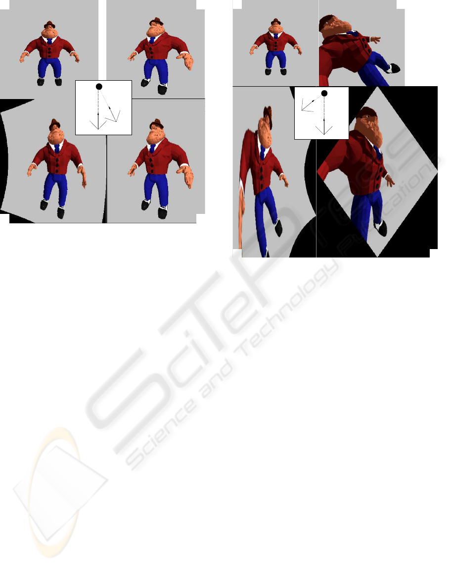
The first example covers the case of one epipole
outside the image at a finite position and the second
epipole lying at infinity (Figure 6). In the second ex-
ample we examine the case of the first epipole lying
inside the image and the second one at infinity (Fig-
ure 7). To show the effect of rotated cameras, which is
likely to occur in an autonomous system, the second
camera of the latter example was rotated 45 degrees.
The figures are arranged to have the same pixel size
in all for sub-images.
Owing to the calculation of the optimum step size
during sampling, a stretching effect is noticeable. For
example, in Figure 6, sub-image a) is sampled along
the left image border in steps less than one pixel to
ensure the distance |c
′
a
′
| of Figure 4 being one pixel.
To match this step size, the right figure was in turn
sampled in steps less than one pixel, thus stretched.
Figure 7 shows the same stretching effect for sim-
ilar reasons. Additionally, the rectified sub-image d)
takes a diamond form. This happens because the sec-
ond camera was rotated 45 degrees along the camera
direction. So, the sampling occurred along a diago-
nal line. The rectified sub-image c) of Figure 7 shows
what happens if an epipole lies inside an image. The
half-lines are sampled in such a way that their begin-
ning, which is the epipole, always is placed on the left
side of the rectified image.
Summarized, rectified images such as those
shown in figures 6 and 7 (parts c) and d)) provide
the possibility of a fast calculation of correspondences
between their source images (such as those shown in
parts a) and b)). The former method of polar recti-
fication would fail to produce these rectified images
in both examples as one epipole of the source images
is positioned at infinity. Using an image homography
would succeed in the first example but fail in the sec-
ond one, because parts of the rectified image would be
mapped to infinity, as one of the epipoles lies inside
the image.
5 CONCLUSION
An extension of the polar rectification process was
presented, covering the special cases where the
ICINCO 2007 - International Conference on Informatics in Control, Automation and Robotics
278

cam 2
cam 1
a) b)
c) d)
e)
Figure 6: One epipole at infinity. a) First image recorded
with camera 1 as shown in e). Its epipole lies outside the
image at a finite position. b) Second image recorded with
camera 2 as shown in e). Its epipole lies at infinity. c) and
d) are rectified versions of images a) and b), respectively,
which have been generated with the proposed method.
epipole of at least one image to be rectified lies at in-
finity. Additionally, the technique of line transfer used
in the original paper of Pollefeys was substituted by
the use of the fundamental matrix alone.
Given the proposed extension of the rectification
process, it is now possible to deal with general cam-
era positions, where former methods failed in special
cases. As even extreme camera positions of an ac-
quisition system can be evaluated now, e.g., for 3D
reconstruction in an object acquisition system, this
opens new possibilities for more flexible autonomous
systems, where successive camera positions are un-
predictable.
ACKNOWLEDGEMENTS
This research was funded by the German Research
Association (DFG) under Grant PE 887/3-1.
cam 1
cam 2
a) b)
c) d)
e)
Figure 7: One epipole inside the image, one at infinity. a)
First image recorded with camera 1 as shown in e). Its
epipole lies inside the image. b) Second image recorded
with camera 2 as shown in e). Its epipole lies at infinity.
c) and d) are rectified versions of images a) and b), respec-
tively, generated with the proposed method.
REFERENCES
Hartley, R. I. and Zisserman, A. (2004). Multiple View Ge-
ometry in Computer Vision. Cambridge University
Press, ISBN: 0521540518, second edition.
Laveau, S. and Faugeras, O. D. (1996). Oriented projec-
tive geometry for computer vision. In ECCV ’96:
Proceedings of the 4th European Conference on Com-
puter Vision-Volume I, pages 147–156, London, UK.
Springer.
Peters, G. (2006). A Vision System for Interactive Object
Learning. In IEEE International Conference on Com-
puter Vision Systems (ICVS 2006), New York, USA.
Pollefeys, M., Koch, R., and van Gool, L. J. (1999). A sim-
ple and efficient rectification method for general mo-
tion. In Proc. International Conference on Computer
Vision (ICCV 1999), pages 496–501.
EXTENSION OF THE GENERALIZED IMAGE RECTIFICATION - Catching the Infinity Cases
279