
A DISTRIBUTED REINFORCEMENT LEARNING CONTROL
ARCHITECTURE FOR MULTI-LINK ROBOTS
Experimental Validation
Jose Antonio Martin H.
Dep. Sistemas Inform
´
aticos y Computaci
´
on, Universidad Complutense de Madrid
C. Prof. Jos
´
e Garc
´
ıa Santesmases, 28040, Cuidad Univesitaria, Madrid, Spain
Javier de Lope
Dept. Applied Intelligent Systems, Universidad Polit
´
ecnica de Madrid
Campus Sur, Ctra. Valencia, km. 7, 28031 Madrid, Spain
Keywords:
Reinforcement Learning, Multi-link Robots, Multi-Agent systems.
Abstract:
A distributed approach to Reinforcement Learning (RL) in multi-link robot control tasks is presented. One of
the main drawbacks of classical RL is the combinatorial explosion when multiple states variables and multiple
actuators are needed to optimally control a complex agent in a dynamical environment. In this paper we
present an approach to avoid this drawback based on a distributed RL architecture. The experimental results
in learning a control policy for diverse kind of multi-link robotic models clearly shows that it is not necessary
that each individual RL-agent perceives the complete state space in order to learn a good global policy but
only a reduced state space directly related to its own environmental experience. The proposed architecture
combined with the use of continuous reward functions results of an impressive improvement of the learning
speed making tractable some learning problems in which a classical RL with discrete rewards (-1,0,1) does
not work.
1 INTRODUCTION
Reinforcement Learning (RL) (Sutton and Barto,
1998) is a paradigm of Machine Learning (ML) that
consists in guiding the learning process by rewards
and punishments.
One of the most important breakthroughs in RL
was the development of Q-Learning (Watkins, 1989).
In a simple form its learning rule is:
Q(s, a) = Q(s, a) + α[r+ γmax
a
Q(s
t+1
, ∗) − Q(s, a)]
(1)
Note that this is the classical moyenne adaptive mod-
ifi
´
ee technique (Venturini, 1994) which adaptively ap-
proximates the average µ of a set x = (x
1
...x
∞
) of ob-
servations:
µ = µ+ α[x
t
− µ], (2)
thus replacing the factor x
t
in (2) with the current re-
ward r plus a fraction γ ∈ (0, 1] of the best possible ap-
proximation to the maximum future expected reward
max
a
Q(s
t+1
, ∗):
µ = µ+ α[r+ γmax
a
Q(s
t+1
, ∗) − µ], (3)
we are indeed approximating the average of the max-
imum future reward when taking the action a at the
state s.
In (Watkins and Dayan, 1992) the authors proved
convergence of Q-Learning to an optimal control pol-
icy with probability 1 under certain single assump-
tions see (Sutton and Barto, 1998, p.148).
In this paper we present a distributed approach to
RL in robot control tasks. One of the main draw-
backs of classical RL is the combinatorial explo-
sion when multiple states variables and multiple ac-
tuators are needed to optimally control a complex
agent in a complex dynamical environment. As
an example, a traditional RL system for the con-
trol of a robot with multiple actuators (i.e. multi-
link robots, snake-like robots, industrial manipula-
tors, etc.) when the control task relies on feedback
from the actuators. This situation produces a huge
table of states× actions pairs which, in the best case,
assuming enough memory to store the table, the learn-
ing algorithm needs a huge amount of time to con-
verge, indeed the problem could become intractable.
192
Antonio Martin H. J. and de Lope J. (2007).
A DISTRIBUTED REINFORCEMENT LEARNING CONTROL ARCHITECTURE FOR MULTI-LINK ROBOTS - Experimental Validation.
In Proceedings of the Fourth International Conference on Informatics in Control, Automation and Robotics, pages 192-197
DOI: 10.5220/0001621201920197
Copyright
c
SciTePress
Also, for some nonlinear parameterized function ap-
proximators, any temporal-difference (TD) learning
method (including Q-learning and SARSA) can be-
come unstable (parameters and estimates going to in-
finity) (Tsitsiklis and Roy, 1996). For the most part,
the theoretical foundation that RL adopts from dy-
namic programming is no longer valid in the case
of function approximation (Sutton and Barto, 1998).
For these reasons the development of distributed algo-
rithms relying on partial observations of states and in-
dividual action selections mechanisms becomes cru-
cial to solve such intractable problems.
Our approach avoids this drawback based on a dis-
tributed architecture. The work is based on the hy-
pothesis that such complex agents can be modeled as
a colony of single interacting agents with single state
spaces as well as single action spaces. This hypothe-
sis is verified empirically by the means of clear exper-
imental results showing the viability of the presented
approach.
The rest of the paper is organized as follows. First
we introduce some previous works on RL for robot
controlling. In the next section we present the basis
of our distributed RL control approach, including a
pseudo-code of the proposed algorithm. Next we de-
fine an application framework in which we have car-
ried out the experiments. For the experiments we use
two multi-link robot models, a three-link planar robot
and an industrial SCARA.
2 RL IN ROBOT CONTROL
RL has been applied successfully to some robot
control task problems (Franklin, 1988; Lin, 1993;
Mataric, 1997; Rubo et al., 2000; Yamada et al., 1997;
Kretchmar, 2000; Kalmar et al., 2000; El-Fakdi et al.,
2005) and is one of the most promising paradigms
in robot learning. This is mainly due to its simplic-
ity. The main advantages of RL over other methods
in robot learning and control are:
1. There is no need to know a prior model of the en-
vironment. This is a crucial advantage because in
most complex tasks a model of the environment is
unknown or is too complex to describe.
2. There is no need to know previously what actions
for each situation must be presented to the learner.
3. The learning process is online by directly interact-
ing with the environment.
4. It is capable of learning from scratch.
RL can be applied to robot control tasks in a very
easy way. The basic elements of a RL learning system
are:
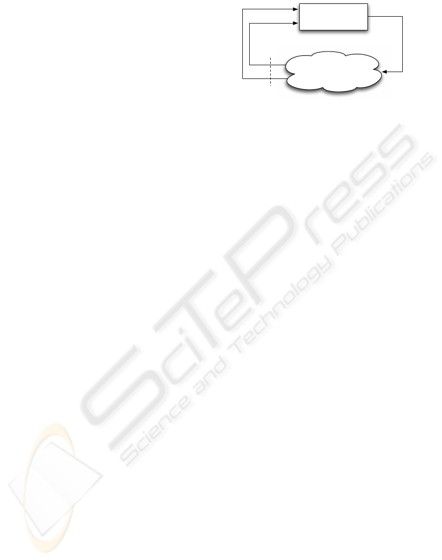
Environment
Agent
state
s
t
reward
r
t
action
a
t
r
t+1
s
t+1
Figure 1: The basic model of an RL system.
1. An agent or a group of agents (i.e. mobile robots)
that perceives the environment (typically called
state S
t
) and behaves on the environment produc-
ing actions (a
t
).
2. The environment in which the agents live, that
could be a simulated world or the real world.
3. A reward signal r
t
that represents the evaluation
of the state and it is used by the agents to evaluate
its behavioral policies.
Fig. 1 shows the agent-environment interaction in
RL. The control cycle can be used directly to control
any robotic task where the agent represents a robot.
The majority of RL algorithms rely on the condi-
tion that the state signal S
t
fulfills the Markov prop-
erty that is, the signal S
t
must contain for the time
step (t) all the information needed to take an optimal
action at time step (t). In other words we can define
that a signal state S
t
fulfills the Markov property if and
only if there is no information that could be added into
S
t
that could produce a more optimal action than the
original signal control.
We use SARSA as the basis for our RL algorithm.
SARSA has been proved to converge under the same
set of single assumptions that Q-Learning (Sutton
and Barto, 1998) but empirically it outperforms the
Q-Learning’s performance. The pseudo-code of the
SARSA algorithm is described in Fig. 2 which uses a
slight variation of the learning rule shown in (1).
3 PROPOSED ARCHITECTURE
In this work we propose a distributed architecture for
RL in order to prevent the combinatorial explosion
when multiple states and actuators are needed. The
main feature of this architecture is the division of the
learning problem into different agents each one for
every different actuator (i.e. joint or motor). Fig. 3
shows the basic control cycle of this architecture.
A DISTRIBUTED REINFORCEMENT LEARNING CONTROL ARCHITECTURE FOR MULTI-LINK ROBOTS -
Experimental Validation
193
———————————————————————
Initialize Q arbitrarily
Repeat( for each episode )
Observe s
Select a for s by ε-greedy policy
Repeat( for n steps )
Take action a, observe r,s
′
Select a
′
for s
′
by ε-greedy policy
Q(s, a) = Q(s, a) + α[r+ γQ(s
′
, a
′
) − Q(s, a)]
s = s
′
;a = a
′
until s is terminal
———————————————————————
Figure 2: SARSA: RL control algorithm.
Agent
Environment
Agent
state
s
t
(i)
reward
r
t
action
a
t
(i)
r
t+1
s
t+1
(i)
Agent
1
i
n
n
n
Figure 3: The basic model of the Distributed Approach to
RL.
In Fig.3 we can see that the RL signal r
t
is the
same for all agents and the state signal s
t+1
is propa-
gated against all agents despite each individual agent
can filter it and use only the information needed to
behave properly. Also, we must note that each agent
emits a different action to the environment. Thus,
each agent will have its own independent memory in
which to store its respective knowledge and hence the
quantity of state-action pairs in the global system is
considerably less than within a full state-action space
due to the additive scheme instead of the multiplica-
tive scheme which is the main cause of the curse of
dimensionality. Fig. 4 shows the proposed algorithm
based on the SARSA algorithm which reflects the
proposed multi-agent control architecture.
Within this distributed approach every agent will
have its own Q-table Q
i
and its own perceptions f
i
(s
i
).
In the case of multi-link robots, each agent will per-
ceive as its own state signal only the current state of
its respective actuator plus the information of the goal
reaching index.
3.1 Continuous Rewards
Traditionally RL systems work with discrete rewards
(i.e. [-1, 0, 1]) but this is not mandatory due to the
algorithms actually can handle scalar reward signals.
———————————————————————
Initialize Q
i
arbitrarily ; ∀i = 1, ..., n
Repeat( for each episode )
Observe (s
1
, ..., s
n
)
Select a
i
for s
i
by ε-greedy policy ; ∀i = 1, ..., n
Repeat( for J steps )
Take actions a
1
, ..., a
n
, observe r, s
′
1
, ..., s
′
n
Select a
′
i
for s
′
i
by ε-greedy policy ; ∀i = 1, ..., n
Q
i
(s
i
, a
i
) = Q
i
(s
i
, a
i
) + α[r+ γQ(s
′
i
, a
′
i
) − Q(s
i
, a
i
)]
s
i
= s
′
i
;a
i
= a
′
i
until s is terminal
———————————————————————
Figure 4: MA-SARSA: A Multi-agent RL control algo-
rithm.
Indeed the conditions for proper convergence assume
scalar rewards signals. In our model we use contin-
uous rewards functions as a way to improve conver-
gence and learning speed. The use of continuous re-
wards signals may lead to some local optima traps but
the exploratory nature of RL algorithms tends to es-
cape from these traps.
One elegant way to formulate a continuous reward
signal in the task of reaching a goal is simply to use
the inverse Euclidean distance plus 1 as shown in (4):
reward =
β
1+ d
n
, (4)
where β is a scalar that controls the absolute magni-
tude of the reward, d is the Euclidean distance from
the goal position and n is an exponent which is used
to change the form in which the function responds to
changes in the Euclidean distance. In out model we
use generally (4) as the reward when the state is termi-
nal and the goal is reached otherwise we use another
continuous function as a penalty function for every
action that does not reach the goal as shown in (5).
punishment = −βd
n
− ε, (5)
where the term ε is used to include some constraints
that the system engineer considers appropriate.
We have used this same kind of continuous re-
wards functions in past works with successful results
for multi-objective RL systems (Martin-H. and De-
Lope, 2006).
4 EXPERIMENTAL
APPLICATION FRAMEWORK
Experiments have been realized on two multi-link
robot models: a three-link planar robot and a SCARA
robot. The experiments are made with the intention
that the robots learn their inverse kinematics in order
ICINCO 2007 - International Conference on Informatics in Control, Automation and Robotics
194
to reach a desired configuration in the joint and Carte-
sian spaces. For this reason we have selected both
types of manipulators.
4.1 Three-Link Planar Robot
The three link planar robot is a configuration which
is generally studied by the Robotics community and
its kinematics is well-known. It includes some re-
dundancy in the calculus of the inverse kinematics by
means of analytic procedures. For this reason, it is
very interesting for the verification of our methods
in this kind of mechanical structures. As we have
commented previously the same approach could be
applied for controlling the movement and body coor-
dination of snake-like robots.
Fig. 5 shows a diagram of the robot model
1
. Its
Denavit-Hartenberg parameters are described in the
Table 1 and its direct kinematic equation is defined
in (6).
−25 −20 −15 −10 −5 0 5 10 15 20 25
0
5
10
15
20
25
X
T
=12.53
Y
T
= 7.55
θ
1
= −13
o
θ
2
= −41
o
θ
3
= −90
o
Target position
Figure 5: Three link-planar robot model.
Table 1: Three link planar robot D-H parameters.
i θ
i
d
i
a
i
α
i
1 θ
1
0 a
1
= 8.625 0
2 θ
2
0 a
2
= 8.625 0
3 θ
3
0 a
3
= 6.125 0
T
3
=
C
123
−S
123
0 a
1
C
1
+ a
2
C
12
+ a
3
C
123
S
123
C
123
0 a
1
S
1
+ a
2
S
12
+ a
3
S
123
0 0 1 0
0 0 0 1
,
(6)
where S
123
and C
123
correspond to sin(θ
1
+ θ
2
+ θ
3
)
and cos(θ
1
+ θ
2
+ θ
3
), respectively (and equally for
S
1
, S
12
, C
1
and C
12
), θ
1
, θ
2
and θ
3
define the robot
joint coordinates —θ
1
for the first joint, located near
1
The original model is by Matt Kontz from Walla Walla
College, Edward F. Cross School of Engineering, February
2001.
to the robot base, θ
2
for the middle joint and θ
3
for
the joint situated in the final extreme— and a
1
, a
2
and a
3
correspond to the physical length of every link,
first, second and third, respectively, numbering from
the robot base.
4.2 Scara Robot
The SCARA robot was selected due to it is a widely
used robot in the industry. It has well-known proper-
ties for the use as manufacturing cells assisting con-
veyor belts, electronic equipment composition, weld-
ing tasks, and so on. In this case we are using a real
three dimension robot manipulator so the agents have
to try to reach an objective configuration in a 3D space
being able to generate an approaching real-time tra-
jectory when the agent system is completely trained.
A physical model of the SCARA robot is shown
in Fig. 6. The Denavit-Hartenberg parameters are de-
fined in Table 2 and the direct kinematic matrix is
shown in (7).
−50
−40
−30
−20
−10
0
10
20
30
40
50−50
−40
−30
−20
−10
0
10
20
30
40
50
0
1
2
3
4
5
6
Target position
Figure 6: SCARA robot model.
Table 2: SCARA robot D-H parameters.
i θ
i
d
i
a
i
α
i
1 θ
1
0 a
1
= 20 0
2 θ
2
0 a
2
= 20 π
3 θ
3
0 0 0
4 0 d
4
0 0
T
4
=
C
12−3
−S
12−3
0 a
1
C
1
+ a
2
C
12
S
12−3
C
12−3
0 a
1
S
1
+ a
2
S
12
0 0 −1 −d
4
0 0 0 1
,
(7)
where S
12−3
and C
12−3
correspond to sin(θ
1
+ θ
2
−
θ
3
) and cos(θ
1
+ θ
2
− θ
3
), respectively (and equally
for S
1
, S
12
, C
1
and C
12
), θ
1
, θ
2
, θ
3
and d
4
are the joint
parameters for the shoulder, elbow, wrist and pris-
matic joints, respectively, and a
1
and a
2
the lengths
of the arm links.
A DISTRIBUTED REINFORCEMENT LEARNING CONTROL ARCHITECTURE FOR MULTI-LINK ROBOTS -
Experimental Validation
195
4.3 Experiments Design
The control task consists of to reach a continuously
changing goal position of the robot end-effector by
means of a random procedure. The goal positions are
defined in such a way that they are always reachable
for the robot. Thus, the learning process needs to de-
velop an internal model of the inverse kinematics of
the robot which is not directly injected by the designer
in a aprioristic way. Through the different trials, a
model of the robot inverse kinematics is learned by
the system.
When a goal position is generated, the robot tries
to reach it. Each trial can finish as a success episode,
i.e. the robot reaches the target at a previously deter-
mined time or as a fail episode, i.e. the robot is not
able to adopt a configuration to reach the goal posi-
tion. In both cases the system parameters are updated
using the previously defined method and a new goal
position is randomly generated.
Once the systems parameters have been tuned by
the RL process, the system has learned an inverse
kinematics model of the robot. Such a model can be
used for real time control of the robot. The learning
process duration depends on the initial conditions and
the randomly generated positions since RL relies on
a kind of stochastic search, but as it is shown in the
experimental results this time is very short. We will
comment in detail on the results in the next section.
5 EXPERIMENTAL RESULTS
The test procedure defined above has been applied
to both robots the three-link planar robot and the
SCARA robot. Although the results are very similar
we offer separate results for each robot.
5.1 The Three-link Planar Robot
The three-link planar robot has a relatively simple in-
verse kinematics, although its three rotation axes are
in parallel, generating multiple candidate configura-
tions for the same position and orientation. The learn-
ing system produces extremely good results, finding
a model of the inverse kinematics in 50 episodes in
average, being the best case of 4 episodes. The aver-
age number of episodes is obtained by a sequence of
30 multiple restarting experiments and calculating the
point at which the convergence is achieved for each
run.
Fig. 7 shows the learning curve for this best case.
As we can observe, before the system runs 4 episodes,
the controller converges to the final solution. The
peaks displayed are due to the randomly nature of the
experiment: the vertical axis represents the steps that
were needed to reach the goal, if the new randomly
generated goal is far from the current position, then
more steps will be needed in order to reach the goal
position.
0 10 20 30 40 50 60 70 80 90 100
0
50
100
150
200
250
300
350
400
Episodes
Steps
Learning curve
Figure 7: Learning curve for the three-link planar robot
model for 100 episodes.
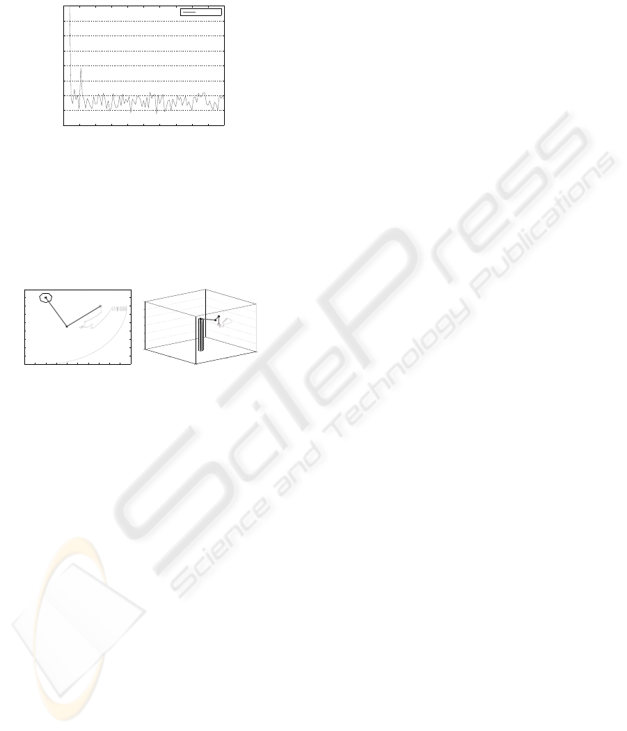
Fig. 8 shows a trace of the behavior of the three-
link planar robot for four consecutive goals, It can be
seen that there is some little noise in the trajectory
in some segments of the paths between consecutive
goals. This noise is the product of the nature of the
goal reaching information due to some zero-crossings
at the orthogonal axes (x,y), this must be interpreted
as search for accuracy in the goal reaching attempt.
We must recall that we are using a mixture of memory
based approach and a reactive mechanism thus these
oscillations are a natural consequence of a reactive be-
havior. This noise can be reduced by some methods
to prevent oscillations in which we are working as a
future improvement.
−25 −20 −15 −10 −5 0 5 10 15 20 25
0
5
10
15
20
25
θ
1
= −15
o
X
T
=13.6
θ
2
= −90
o
Y
T
= 0.79
θ
3
= −45
o
φ
T
= −60
o
Episodes: 5
1
2
3
4
Figure 8: Trace for the three-link planar robot for four con-
secutive goals.
5.2 The Scara Robot
The SCARA robot presents very similar results.
Fig. 9 shows a learning curve for 100 episodes. In
these cases the learning process converges slower than
the one of previous robot. The abrupt peaks that ap-
pears in the first episodes show the adaptation pro-
ICINCO 2007 - International Conference on Informatics in Control, Automation and Robotics
196
cess (learning). For the SCARA robot 67 episodes
are needed as average to find a solution, obtaining a
best case after 23 episodes.
0 10 20 30 40 50 60 70 80 90 100
0
50
100
150
200
250
300
350
400
Episodes
Steps
Learning curve
Figure 9: Learning curve for the SCARA robot model for
100 episodes.
Fig. 10 shows a trace of the behavior of the
SCARA robot for four consecutive goals, in this pic-
ture the same oscillations can be seen as in the trace
of the three-link planar robot due to the zero-crossing
effect explained above.
−5
0
5
10
15
20
25
30
35
40
−10 −5 0 5 10 15 20 25 30 35 40
1
2
3
4
−50
0
50
−50
0
50
0
1
2
3
4
5
6
1
2
3
4
Figure 10: Trace for the SCARA robot for four consecutive
goals.
6 CONCLUSIONS
A distributed approach to RL in robot control tasks
has been presented. To verify the method we have de-
fined an experimental framework and we have tested
it on two well-known robotic manipulators: a three-
link planar robot and an industrial SCARA.
The experimental results in learning a control
policy for diverse kind of multi-link robotic models
clearly shows that it is not necessary that the indi-
vidual agents perceive the complete state space in or-
der to learn a good global policy but only a reduced
state space directly related to its own environmental
experience. Also we have shown that the proposed
architecture combined with the use of continuous re-
ward functions results in an impressive improvement
of the learning speed making tractable some learn-
ing problems in which a classical RL with discrete
rewards (−1, 0, 1) does not work. Also we want to
adapt the proposed method to snake-like robots. The
main drawback in this case could be the absence of a
base which fixes the robot to the environment and its
implication in the definition of goal positions.
ACKNOWLEDGEMENTS
This work has been partially funded by the Span-
ish Ministry of Science and Technology, project
DPI2006-15346-C03-02.
REFERENCES
El-Fakdi, A., Carreras, M., and Ridao, P. (2005). Direct
gradient-based reinforcement learning for robot be-
havior learning. In ICINCO 2005, pages 225–231.
INSTICC Press.
Franklin, J. A. (1988). Refinement of robot motor skills
through reinforcement learning. In Proc. of 27
th
Conf.
on Decision and Control, pages 1096–1101, Austin,
Texas.
Kalmar, Szepesvari, and Lorincz (2000). Modular rein-
forcement learning: A case study in a robot domain.
ACTACYB: Acta Cybernetica, 14.
Kretchmar, R. M. (2000). A synthesis of reinforcement
learning and robust control theory. PhD thesis, Col-
orado State University.
Lin, L.-J. (1993). Scaling up reinforcement learning for
robot control. Machine Learning.
Martin-H., J. A. and De-Lope, J. (2006). Dynamic goal co-
ordination in physical agents. In ICINCO 2006, pages
154–159. INSTICC Press.
Mataric, M. J. (1997). Reinforcement learning in the multi-
robot domain. Auton. Robots, 4(1):73–83.
Rubo, Z., Yu, S., Xingoe, W., Guangmin, Y., and Guochang,
G. (2000). Research on reinforcement learning of the
intelligent robot based on self-adaptive quantization.
In Proc. of the 3rd World Congr. on Intelligent Con-
trol and Automation. IEEE, Piscataway, NJ, USA, vol-
ume 2, pages 1226–9.
Sutton, R. S. and Barto, A. G. (1998). Reinforcement Learn-
ing, An Introduction. The MIT press.
Tsitsiklis, J. N. and Roy, B. V. (1996). Analysis of temporal-
diffference learning with function approximation. In
Mozer, M., Jordan, M. I., and Petsche, T., editors,
NIPS, pages 1075–1081. MIT Press.
Venturini, G. (1994). Adaptation in dynamic environments
through a minimal probability of exploration. In
SAB94, pages 371–379, Cambridge, MA, USA. MIT
Press.
Watkins, C. J. (1989). Models of Delayed Reinforcement
Learning. PhD thesis, Psychology Department, Cam-
bridge University, Cambridge, United Kingdom.
Watkins, C. J. and Dayan, P. (1992). Technical note Q-
learning. Machine Learning, 8:279.
Yamada, S., Watanabe, A., and Nakashima, M. (1997).
Hybrid reinforcement learning and its application to
biped robot control. In NIPS. The MIT Press.
A DISTRIBUTED REINFORCEMENT LEARNING CONTROL ARCHITECTURE FOR MULTI-LINK ROBOTS -
Experimental Validation
197
