
SMARTMOBILE – AN ENVIRONMENT FOR GUARANTEED
MULTIBODY MODELING AND SIMULATION
Ekaterina Auer and Wolfram Luther
IIIS, University of Duisburg-Essen, Lotharstr. 63, Duisburg, Germany
Keywords:
Validated method, interval, Taylor model, initial value problem, guaranteed multibody modeling and simula-
tion.
Abstract:
Multibody modeling and simulation is important in many areas of our life from a computer game to space ex-
ploration. To automatize the process for industry and research, a lot of tools were developed, among which the
program MOBILE plays a considerable role. However, such tools cannot guarantee the correctness of results,
for example, due to possible errors in the underlying finite precision arithmetic. To avoid such errors and si-
multaneously prove the correctness of results, a number of so called validated methods were developed, which
include interval, affine and Taylor form based arithmetics. In this paper, we present the recently developed
multibody modeling and simulation tool SMARTMOBILE based on MOBILE, which is able to guarantee
the correctness of results. The use of validated methods there allows us additionally to take into account the
uncertainty in measurements and study its influence on simulation. We demonstrate the main concepts and
usage with the help of several mechanical systems, for which kinematical or dynamic behavior is simulated in
a validated way.
1 INTRODUCTION
Modeling and simulation of kinematics and dynamics
of mechanical systems is employed in many branches
of modern industry and applied science. This fact
contributed to the appearance of various tools for au-
tomatic generation and simulation of models of multi-
body systems, for example, MOBILE (Kecskem
´
ethy,
1993). Such tools produce a model (mostly a system
of differential or algebraic equations or both) from
a formalized description of the goal mechanical sys-
tem. The system is then solved using a correspond-
ing numerical algorithm. However, the usual imple-
mentations are based on finite precision arithmetic,
which might lead to unexpected errors due to round
off and similar effects. For example, unreliable nu-
merics might ruin an election (German Green Party
Convention in 2002) or cost people lives (Patriot Mis-
sile failure during the Golf War), cf. (Huckle, 2005).
Aside from finite precision errors, possible mea-
surement uncertainties in model parameters and er-
rors induced by model idealization encourage the em-
ployment of a technique called interval arithmetic and
its extensions in multibody modeling and simulation
tools. Essential ideas of interval arithmetic were de-
veloped simultaneously and independently by several
people whereas the most influential theory was for-
mulated by R. E. Moore (Moore, 1966). Instead of
providing a point on the real number axis as an (in-
exact) answer, intervals supply the lower and upper
bounds that are guaranteed to contain the true result.
These two numbers can be chosen so as to be ex-
actly representable in a given finite precision arith-
metic, which cannot be always ensured in the usual
finite precision case. The ability to provide a guar-
anteed result supplied a name for such techniques –
”validated arithmetics”. Their major drawback is that
the output might be too uncertain (e.g. [−∞;+∞]) to
provide a meaningful answer. Usually, this is an in-
dication that the problem might be ill conditioned or
inappropriately formulated, and so the finite precision
result wrong.
To minimize the possible influence of overestima-
tion on the interval result, this technique was extended
109
Auer E. and Luther W. (2007).
SMARTMOBILE – AN ENVIRONMENT FOR GUARANTEED MULTIBODY MODELING AND SIMULATION.
In Proceedings of the Fourth International Conference on Informatics in Control, Automation and Robotics, pages 109-116
DOI: 10.5220/0001624601090116
Copyright
c
SciTePress

with the help of such notions as affine (de Figueiredo
and Stolfi, 2004) or Taylor forms/models (Neumaier,
2002). Besides, strategies and algorithms much less
vulnerable to overestimation were developed. They
include rearranging expression evaluation, coordinate
transformations, or zonotopes (Lohner, 2001).
The second focus in this paper is MOBILE, an
object oriented C++ environment for modeling and
simulation of kinematics and dynamics of mechani-
cal systems based on the multibody modeling method.
Its central concept is a transmission element which
maps motion and force between system states. For
example, an elementary joint modeling revolute and
prismatic joints is such a transmission element. Me-
chanical systems are considered to be concatenations
of these entities. In this way, serial chains, tree type
or closed loop systems can be modeled. With the
help of the global kinematics, the transmission func-
tion of the complete system chain can be obtained
from transmission functions of its parts. The inverse
kinematics and the kinetostatic method (Kecskem
´
ethy
and Hiller, 1994) help to build dynamic equations of
motion, which are solved with common initial value
problem (IVP) solvers. MOBILE belongs to the nu-
merical type of modeling software, that is, it does
not produce a symbolic description of the resulting
model. Only the values of output parameters for the
user-defined values of input parameters and the source
code of the program itself are available.
SMARTMOBILE (S
imulation and Modeling of
dynA
mics in MOBILE: Reliable and Template
based) enhances the usual, floating point based
MOBILE with validated arithmetics and IVP
solvers (Auer et al., 2006a). In this way, it can model
and perform validated simulation of the behavior of
various classes of mechanical systems including non-
autonomous and closed-loop ones as well as provide
more realistic models by taking into account the un-
certainty in parameters.
In this paper, we give an overview of the struc-
ture and the abilities of SMARTMOBILE. First, the
main validated techniques and software are refer-
enced briefly in Section 2. In Section 3, the main
features of MOBILE are described in short to pro-
vide a better understanding of the underlying struc-
ture of SMARTMOBILE. In Section 4, we describe
the implementation of SMARTMOBILE in some de-
tail and validate kinematical and dynamic behavior of
several example systems with the help of this environ-
ment. We summarize the paper in Section 5. On the
whole, we give an overview of the potential of vali-
dated methods in mechanical modeling, and, in par-
ticular, the potential of SMARTMOBILE.
2 VALIDATED METHODS AND
SOFTWARE
To guarantee the correctness of MOBILE results, it
is necessary to enhance this tool with validated con-
cepts. Fortunately, we do not need to implement these
concepts from scratch. In the last decades, various li-
braries were implemented that supported different as-
pects of validated calculus. In the first Subsection, we
name several of these tools. After that, we give a very
brief overview of interval arithmetic and an algorithm
for solving IVPs (initial value problems) to provide a
reference about the difference of validated methods to
the usual floating point ones.
2.1 Validating Multibody Tools of the
Numerical Type
To validate the results of multibody modeling and
simulation software of the numerical type, the
following components are necessary. First, the
means are required to work with arithmetic op-
erations and standard functions such as sine or
cosine in a guaranteed way. Here, the basic
principles of interval calculus and its extensions
are used. Interval arithmetic is implemented in
such libraries as PROFIL/BIAS (Kn
¨
uppel, 1994),
FILIB++ (Lerch et al., 2001), C-XSC (Klatte et al.,
1993). LIBAFFA (de Figueiredo and Stolfi, 2004) is
a library for affine arithmetic, whereas COSY (Berz
and Makino, 2002) implements Taylor models.
Second, validated algorithms for solving sys-
tems of algebraic, differential or algebraic-differential
equations are necessary. C-XSC TOOLBOX (Ham-
mer et al., 1995) offers a general means of solving dif-
ferent classes of systems as well as an implementation
in C-XSC. For IVP solving in interval arithmetic,
there exist such packages as AWA (Lohner, 1988),
VNODE (Nedialkov, 2002), and recently developed
VALENCIA-IVP (Auer et al., 2006a). In the frame-
work of Taylor models, the solver COSY VI (Berz
and Makino, 1998) was developed.
Finally, almost all of the above mentioned solvers
need means of computing (high order) derivatives au-
tomatically. Some of them, for example, COSY VI,
use the facilities provided by the basis arithmetic in
COSY. Interval implementations do not possess this
facility in general; external tools are necessary in this
case. The symbolic form of the mathematical model,
which is necessary to be able to obtain derivatives au-
tomatically, is not available in case of software of the
numerical type. However, a method called algorith-
mic differentiation (Griewank, 2000) offers a possi-
bility to obtain the derivatives using the code of the
ICINCO 2007 - International Conference on Informatics in Control, Automation and Robotics
110

program itself.
There are two main techniques to implement al-
gorithmic differentiation of a piece of program code:
overloading and code transformation. In the first case,
a new data type is developed that is capable of com-
puting the derivative along with the function value.
This new data type is used instead of the simple one
in the code piece. The drawback of this method is the
lack of automatic optimization during the derivative
computation. FADBAD++ (Stauning and Bendtsen,
2005) is a generic library implementing this approach
for arbitrary user-defined basic data types. The tech-
nique of code transformation presupposes the devel-
opment of a compiler that takes the original code
fragment and the set of differentiation rules as its
input and produces a program delivering derivatives
as its output. This approach might be difficult to
implement for large pieces of code which are self-
contained programs themselves. However, derivatives
can be evaluated more efficiently with this technique.
An implementation is offered in the library ADOL-
C (Griewank et al., 1996).
This list of tools is not supposed to be com-
plete. All of the above mentioned packages are im-
plemented (or have versions) in C++, an important
criterium from our point of view since MOBILE is
also implemented in this language.
2.2 Theory Overview
In this Subsection, we consider the basic principles of
validated computations using the example of interval
arithmetic. First, elementary operations in this arith-
metic are described. Then a basic interval algorithm
for solving IVPs is outlined to give an impression of
the difference to floating point analogues. In particu-
lar, the latter passage makes clear why automatic dif-
ferentiation is unavoidable while simulating dynam-
ics of mechanical systems, that is, solving systems of
differential equations.
An interval [x
;x], where x is the lower, x the up-
per bound, is defined as [x
;x] = {x ∈ R : x ≤ x ≤ x}.
For any operation ◦ = {+, −, ·, /} and intervals [x
;x],
[y
;y], the corresponding interval operation can be de-
fined as [x
;x] ◦ [y;y] =
[min(x
◦ y, x◦ y,x◦ y, x◦ y);max(x ◦ y, x◦ y,x ◦ y, x◦ y))] .
Note that the result of an interval operation is also an
interval. Every possible combination of x ◦ y, where
x ∈ [x;x] and y ∈ [y;y], lies inside this interval. (For
division, it is assumed that 0 /∈ [y
;y].)
To be able to work with this definition on a com-
puter using a finite precision arithmetic, a concept of
a machine interval is necessary. The machine interval
has machine numbers as the lower and upper bounds.
To obtain the corresponding machine interval for the
real interval [x
;x], the lower bound is rounded down to
the largest machine number equal or less than x
, and
the upper bound is rounded up to the smallest machine
number equal or greater than x.
Consider an algorithm for solving the IVP
˙x(t) = f(x(t)), x(t
0
) ∈ [x
0
],
(1)
where t ∈ [t
0
,t
n
] ⊂ R for some t
n
> t
0
, f ∈ C
p−1
(
D )
for some p > 1,
D ⊆ R
m
is open, f : D 7→ R
m
,
and [x
0
] ⊂
D . The problem is discretized on a
grid t
0
< t
1
< ··· < t
n
with h
k−1
= t
k
− t
k−1
. De-
note the solution with the initial condition x(t
k−1
) =
x
k−1
by x(t;t
k−1
,x
k−1
) and the set of solutions
{x(t;t
k−1
,x
k−1
) | x
k−1
∈ [x
k−1
]} by x(t;t
k−1
,[x
k−1
]).
The goal is to find interval vectors [x
k
] for which the
relation x(t
k
;t
0
,[x
0
]) ⊆ [x
k
], k = 1,...,n holds.
The (simplified) kth time step of the algorithm
consists of two stages (Nedialkov, 1999) :
1. Proof of existence and uniqueness.
Compute a step
size h
k−1
and an a priori enclosure [ ˜x
k−1
] of the solu-
tion such that
(i) x(t;t
k−1
,x
k−1
) is guaranteed to exist for all t ∈
[t
k−1
;t
k
] and all x
k−1
∈ [x
k−1
],
(ii) the set of solutions x(t;t
k−1
,[x
k−1
]) is a subset of
[ ˜x
k−1
] for all t ∈ [t
k−1
;t
k
].
Here, Banach’s fixed-point theorem is applied to the
Picard iteration.
2. Computation of the solution.
Compute a tight en-
closure [x
k
] ⊆ [ ˜x
k−1
] of the solution of the IVP such
that x(t
k
;t
0
,[x
0
]) ⊆ [x
k
]. The prevailing algorithm is
as follows.
2.1. Choose a one-step method
x(t;t
k
,x
k
) = x(t;t
k−1
,x
k−1
) + h
k−1
ϕ(x(t;t
k−1
,x
k−1
)) + z
k
,
where ϕ(·) is an appropriate method function, and z
k
is the local error which takes into account discretiza-
tion effects. The usual choice for ϕ(·) is a Taylor se-
ries expansion.
2.2. Find an enclosure for the local error z
k
. For
the Taylor series expansion of order p − 1, this en-
closure is obtained as [z
k
] = h
p
k−1
f
[p]
([ ˜x
k−1
]), where
f
[p]
([ ˜x
k−1
]) is an enclosure of the pth Taylor coeffi-
cient of the solution over the state enclosure [ ˜x
k−1
]
determined by the Picard iteration in Stage One.
2.3. Compute a tight enclosure of the solution. If
mean-value evaluation for computing the enclosures
of the ranges of f
[i]
([x
k
]), i = 1, ..., p − 1, instead of
the direct evaluation of f
[i]
([x
k
]) is used, tighter en-
closures can be obtained.
Note that Taylor coefficients and their Jacobians (used
in the mean-value evaluation) are necessary to be able
to use this algorithm.
SMARTMOBILE – AN ENVIRONMENT FOR GUARANTEED MULTIBODY MODELING AND SIMULATION
111

3 MOBILE
A transmission element, the basis of MOBILE, maps
motion and loads between state objects (coordinate
frames or variables) according to
q
′
= φ(q), ˙q
′
= J
φ
˙q,
¨q
′
= J
φ
¨q+
˙
J
φ
˙q, Q = J
T
φ
Q
′
.
(2)
J
φ
is the Jacobian of φ, the mapping for the motion
transmission. Other characteristics are vectors of di-
mension depending on the degrees of freedom of a
mechanical system. Here, q and q
′
are the general-
ized positions, ˙q and ˙q
′
the velocities, ¨q and ¨q
′
the
accelerations, as well as Q and Q
′
the forces of the
transmission element in the original and final states,
respectively. The transmission of force is assumed to
be ideal. That is, power is neither generated nor con-
sumed.
Models in MOBILE are concatenations of trans-
mission elements. The overall mapping of this con-
catenation from the original state into the final one
is obtained by the composition of the corresponding
mappings of the intermediate states. Concatenated el-
ements are considered as a single transmission ele-
ment. This helps to solve the task of the global kine-
matics: to obtain the positions, the orientations, the
velocities, and the accelerations of all bodies of a me-
chanical system from the given q, ˙q, and ¨q.
All transmission elements are derived from the ab-
stract class
MoMap
, which supplies their main func-
tionality including the methods
doMotion()
and
doForce()
for transmission of motion and force.
For example, elementary joints are modeled by the
MoMap
-derived class
MoElementaryJoint
. Besides,
there exist elements for modeling mass properties and
applied forces. The corresponding representations
of the mapping (2) for these elements are described
in (Kecskem
´
ethy, 1993).
Transmission elements are assembled to chains
implemented by the class
MoMapChain
. The methods
doMotion()
and
doForce()
can be used for a chain
representing the system to determine the correspond-
ing composite transmission function.
To model dynamics of a mechanical system, the
equations of motion have to be built and solved. Their
minimal form is given by
M(q;t) ¨q+ b(q, ˙q;t) = Q(q, ˙q;t) , (3)
where M(q;t) is the generalized mass matrix,
b(q, ˙q;t) the vector of generalized Coriolis and cen-
trifugal forces, and Q(q, ˙q;t) the vector of applied
forces. The class
MoEqmBuilder
is responsible for
generation of such equations, that is, computation of
M, b, and Q for each given q, ˙q, and t.
After the introduction of a state vector x =
q
T
, ˙q
T
T
, the state-space form of the state equations
is obtained as
˙x =
˙q
¨q
=
˙q
−M
−1
b
Q
, (4)
where
b
Q(q, ˙q;t) = b(q, ˙q;t) − Q(q, ˙q;t). This is the
responsibility of the class
TMoMechanicalSystem
.
Finally, an IVP corresponding to (4) is
solved by an appropriate integrator algorithm,
for example, Runge–Kutta’s using the class
MoRungeKuttaIntegrator
derived from the
basic class
MoIntegrator
.
MOBILE models and simulates mechanical sys-
tems directly as executable programs. This allows
the user to embed the resulting modules in existing
libraries easily. Besides, the core of MOBILE is ex-
tendable owing to its open system design.
As already mentioned, MOBILE belongs to the
numerical type of the modeling software, by which
we mean that it does not produce the symbolic de-
scription of the resulting mathematical model, as op-
posed to the symbolical type. In the latter case, the
process of validation of the model is basically reduced
to the application of the validated methods to the ob-
tained system of equations. In the former case, it is
necessary to integrate verified techniques into the core
of the software itself, the task which cannot always
be solved since many modeling tools are not open
source.
4 SMARTMOBILE
In this Section, we first describe the main features of
the recently developed multibody modeling and sim-
ulation tool SMARTMOBILE which produces guar-
anteed results in the constraints of the given model.
There, the modeling itself can be enhanced by tak-
ing into account the uncertainty in parameters, which
might result, for example, from measurements. Af-
ter that, we demonstrate the possibilities SMARTMO-
BILE offers by simulating kinematical and dynamic
behavior of two example systems in a validated way.
4.1 Main Features
The focus of SMARTMOBILE is to model and simu-
late dynamics of mechanical systems in a guaranteed
way. The concept behind MOBILE, however, pre-
supposes that kinematics is also modeled (almost as a
by-product) and so it is easy to simulate it afterwards.
That is why SMARTMOBILE is one of the rare vali-
dated tools that possess both functionalities.
ICINCO 2007 - International Conference on Informatics in Control, Automation and Robotics
112

To simulate dynamics, it is necessary to solve an
IVP for the differential(-algebraic) equations of mo-
tion of the system model in the state space form.
As already mentioned, validated IVP solvers need
derivatives of the right side of these equations. They
can be obtained using algorithmic differentiation, the
method that is practicable but might consume a lot of
CPU time in case of such a large program as MO-
BILE. An alternative is to make use of the system’s
mechanics for this purpose. This option is not pro-
vided by MOBILE developers yet and seems to be
rather difficult to algorithmize for (arbitrary) higher
orders of derivatives. That is why it was decided to
employ the first possibility in SMARTMOBILE.
To obtain the derivatives, SMARTMOBILE uses
the overloading technique. In accordance with
Subsection 2.1, all relevant occurrences of
MoReal
(an alias of
double
in MOBILE) have to be re-
placed with an appropriate new data type. Almost
each validated solver needs a different basic vali-
dated data type. Therefore, the strategy in SMART-
MOBILE is to use pairs type/solver. To pro-
vide interval validation of dynamics with the help
of VNODE-based solver
TMoAWAIntegrator
, the
basic data type
TMoInterval
including data types
necessary for algorithmic differentiation should be
used. The data type
TMoFInterval
enables the use
of
TMoValenciaIntegrator
, an adjustment of the
basic version of VALENCIA-IVP. The newly de-
veloped
TMoRiotIntegrator
is based on the IVP
solver from the library RIOT, an independent C++
version of COSY and COSY VI, and requires
the class
TMoTaylorModel
, a SMARTMOBILE-
compatible wrapper of the library’s own data type
TaylorModel
. Analogously, to be able to use an ad-
justment of COSY VI, the wrapper
RDAInterval
is necessary. Modification of the latter solver for
SMARTMOBILE is currently work in progress.
In general, kinematics can be simulated with
the help of all of the above mentioned basic
data types. However, other basic data types
might become necessary for more specific tasks
such as finding of equilibrium states of a sys-
tem since they require specific solvers. SMART-
MOBILE provides an option of modeling equilib-
rium states in a validated way with the help of
the interval-based data type
MoFInterval
and the
class
MoIGradientStaticEquilibriumFinder
, a
version of the zero-finding algorithm from the C-
XSC TOOLBOX.
The availability of several basic data types in
SMARTMOBILE points out its second feature: the
general data type independency through its template
structure. That is,
MoReal
is actually replaced with a
placeholder and not with a concrete data type. For ex-
ample, the transmission element
MoRigidLink
from
MOBILE is replaced with its template equivalent
TMoRigidLink
, the content of the placeholder for
which (e.g.
TMoInterval
or
MoReal
, cf. Figure 1)
can be defined at the final stage of the system as-
sembly. This allows us to use a suitable pair con-
sisting of the data type and solver depending on the
application at hand. If only a reference about the
form of the solution is necessary,
MoReal
itself and
a common numerical solver (e.g. Runge-Kutta’s) can
be used. If a relatively fast validation of dynamics
without much uncertainty in parameters is of inter-
est,
TMoInterval
and
TMoAWAIntegrator
might be
the choice. For validation of highly nonlinear systems
with a considerable uncertainty, the slower combina-
tion of
TMoTaylorModel
and
TMoRiOTIntegrator
can be used.
MOBILE SmartMOBILE
TMoRigidLink<TMoInterval> R;
ր
MoRigidLink R;
ց
TMoRigidLink<MoReal> R;
Figure 1: Template usage.
A MOBILE user can easily switch to SMART-
MOBILE because the executable programs for the
models in both environments are similar. In the val-
idated environment, the template syntax should be
used. The names of transmission elements are the
same aside from the preceding letter
T
. The methods
of the classes have the same names, too. Only the
solvers are, of course, different, although they follow
the same naming conventions.
4.2 Examples
First, we give an example of the guaranteed simula-
tion of kinematics of a five arm manipulator, the sys-
tem defined in detail in (Traczinski, 2006). The mod-
eling of the system itself can be enhanced in SMART-
MOBILE by using so called sloppy joints (Traczin-
ski, 2006) instead of usual revolute ones. In the trans-
mission element responsible for the modeling of the
K
i
K
i+1
ϕ
i
l
i
α
i
body i
body i + 1
F
i+1
= F
i
M
i+1
= M
i
+ l
i
× F
i
Figure 2: A sloppy joint.
SMARTMOBILE – AN ENVIRONMENT FOR GUARANTEED MULTIBODY MODELING AND SIMULATION
113

Table 1: Widths of the position enclosures.
x y CPU (s)
TMoInterval
1.047 1.041 0.02
TMoTaylorModel
0.163 0.290 0.14
sloppy joint, it is no longer assumed that the joint con-
nects the rotational axes of two bodies exactly con-
centrically. Instead, the relative distance between the
axes is supposed to be within a specific (small) range.
Two additional parameters are necessary to describe
the sloppy joint (cf. Figure 2): radius l
i
∈ [0;l
max
]
and the the relative orientation angle α
i
∈ [0;2π) (the
parameter ϕ
i
that describes the relative orientation be-
tween two connected bodies is the same both for the
sloppy and the usual joint).
The considered system consists of five arms of the
lengths l
0
= 6.5m, l
1
= l
2
= l
3
= 4m, and l
4
= 3.5m,
each with the uncertainty of ±1%. The arms are con-
nected with five sloppy joints, for which l
max
= 2mm
and initial angle constellation is ϕ
0
= 60
◦
, ϕ
1
= ϕ
2
=
ϕ
3
= −20
◦
, and ϕ
4
= −30
◦
. Each of these angles has
an uncertainty of ±0.1
◦
.
In Figure 3, left, the (abridged) SMARTMOBILE
model of the manipulator is shown (the system geom-
etry described above is omitted). First, all the nec-
essary coordinate frames are defined with the help of
the array
K
. Analogously, the required rigid links
L
and sloppy joints
R
, with which arms and their con-
nections are modeled, are declared. They are defined
later inside the
for
loop. The array
l
characterizes
the lengths of the rigid links, and
phi
is used to define
the angles of sloppy joints. All elements are assem-
bled into one system using the element
manipulator
.
By calling the method
doMotion()
for this element,
we can obtain the position of the tip of the manipu-
lator, which equals the rotational matrix
R
multiplied
by the translational vector
r
, both stored in the last
coordinate frame
K[10]
.
We simulate kinematics with the help of intervals
and Taylor models. That is, the placeholder
type
is
either
TMoInterval
or
TMoTaylorModel
. Both po-
sition enclosures are shown in Figure 3, right. Note
that enclosures obtained with intervals are wider than
whose obtained with Taylor models (cf. also Table 1,
where the widths of the corresponding intervals are
shown). Taylor models are bounded by intervals to
provide a comparison. Numbers are rounded up to
the third digit after the decimal point. CPU times are
measured on a Pentium 4, 3.0 GHz PC under CYG-
WIN.
The statistic analysis of the same system with
the help of the Monte-Carlo method (Metropolis and
Ulam, 1949) carried out in (H
¨
orsken, 2003) shows
Table 2: Performance of
TMoAWAIntegrator
,
TMoRiOTIntegrator
, and
TMoValenciaIntegrator.
for
the double pendulum over the time interval [0;0.4].
Strategy
AWA RiOT Valencia
Break-down 0.424 0.820 0.504
CPU time 1248 9312 294
that the results, especially those for Taylor mod-
els, are acceptable. Although the set of all possi-
ble positions obtained statistically with the help of
50,000 simulations (solid black area in Figure 3)
is not as large as even the rectangle obtained with
TMoTaylorModel
, there might exist parameter con-
stellations which lead to the results from this rectan-
gle. Besides, statistical simulations require a lot of
CPU time, which is not the case with SMARTMO-
BILE. Additionally, the results are proven to be cor-
rect there through the use of validated methods.
The next example is the double pendulum with an
uncertain initial angle of the first joint from (Auer
et al., 2006a). The lengths of both massless arms
of the pendulum are equal to 1m and the two point
masses amount to 1kg each with the gravitational con-
stant g = 9.81
m
s
2
The initial values for angles (speci-
fied in rad) and angular velocities (in
rad
s
) are given
as
3π
4
−
11π
20
0.43 0.67
T
,
where the initial angle of the first joint has an uncer-
tainty of ±1% of its nominal value.
The interval enclosures of the two angles β
1
and
β
2
of the double pendulum are shown for identical
time intervals in Figure 4. Besides, Table 2 summa-
rizes the results. The line ”Break-down” contains the
time in seconds after which the corresponding method
no longer works. That is, the correctness of results
cannot be guaranteed after that point. This happens
here due to both the chaotic character of the consid-
ered system and the resulting overestimation. The last
line indicates the CPU time (in seconds) which the
solvers take to obtain the solution over the integration
interval [0;0.4]. Note that the CPU times are provided
only as a rough reference since the solvers can be fur-
ther optimized in this respect.
The use of
TMoValenciaIntegrator
improves
both the tightness of the resulting enclosures and the
CPU time in comparison to
TMoAWAIntegrator
for
this example. Although
TMoRiOTIntegrator
breaks
down much later than the both former solvers, it needs
a lot of CPU time.
The double pendulum is a simple example of the
opportunities that SMARTMOBILE offers for dy-
ICINCO 2007 - International Conference on Informatics in Control, Automation and Robotics
114
TMoFrame<type> *K=new TMoFrame<type>[2*5+1];
TMoAngularVariable<type> *phi=new
TMoAngularVariable<type>[5];
TMoVector<type> *l=new TMoVector<type>[5];
TMoSlacknessJoint<type> *R=new
TMoSlacknessJoint<type>[5];
TMoRigidLink<type> *L=new TMoRigidLink<type>[5];
TMoMapChain<type> manipulator;
double l_max;
for(int i=0;i<5;i++){
TMoSlacknessJoint<type> joint(K[2*i],K[2*i+1],
phi[i],zAxis,l_max);
TMoRigidLink<type> link(K[2*i],K[2*i+1],l[i]);
R[i]=joint; L[i]=link;
Manipulator<<R[i]<<L[i];
}
Manipulator.doMotion();
cout<<"Position="<<K[10].R*K[10].r;
(a) SMARTMOBILE model.
Intervalenclosure
Taylormodelenclosure(order5)
16.416.616.81717.217.417.617.8
x(m)
8.4
8.2
8
7.8
7.6
7.4
7.2
y(m)
(b) Enclosures of the position of the tip.
Figure 3: Kinematics of the five arm manipulator with uncertain parameters.
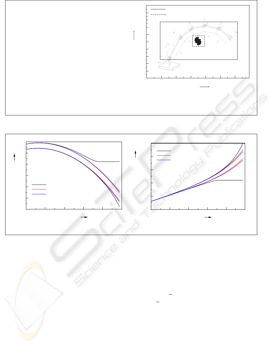
0 0.082 0.164 0.246 0.328 0.41
time (s)
1.8
1.9
2
2.1
2.2
2.3
2.4
first angle (rad)
TMoAWAIntegrator
TMoRiOTIntegrator
TMoValenciaIntegrator
(a) Enclosure of the first joint angle.
0 0.082 0.164 0.246 0.328 0.41
time (s)
-1.8
-1.68
-1.56
-1.44
-1.32
-1.2
second angle (rad)
TMoAWAIntegrator
TMoRiOTIntegrator
TMoValenciaIntegrator
(b) Enclosure of the second joint angle.
Figure 4: Interval enclosures for the first and second state variable of the double pendulum.
namic simulation. More close-to-life examples are
treated in (Auer et al., 2006b), (Auer, 2006), (Auer
et al., 2004).
At last, consider the previous example once again
but without the uncertainty in β
1
. To find equilibrium
states of this system, we use the basic data type
MoFInterval
instead of
TMoInterval
and ap-
ply
MoIGradientStaticEquilibriumFinder
to the element
manipulator
instead of us-
ing
TMoMechanicalSystem
and an integra-
tor. All four possible equilibria (stable and
unstable) are found by the validated solver
MoIGradientStaticEquilibriumFinder
in
the starting interval [−3.15;1] for all coordinates
(shown rounded up to the third digit after the decimal
point):
1: ([-3.142;-3.142];[-3.142;-3.142])
2: ([-3.142;-3.142];[-0.000; 0.000])
3: ([-0.000; 0.000];[-3.142;-3.142])
4: ([-0.000; 0.000];[-0.000; 0.000])
Since we do not have any uncertainties in the model,
the intervals obtained are very close to point intervals,
that is, β
i
≈
β
i
. The difference is noticeable only af-
ter the 12-th digit after the decimal point. However, if
the same problem is modeled using the non-verified
model in MOBILE, only one (unstable) equilibrium
state [β
1
,β
2
] =
[3.142;-3.142]
is obtained (using
the identical initial guess).
5 CONCLUSIONS
In this paper, we presented a recently developed tool
SMARTMOBILE for guaranteed modeling and simu-
SMARTMOBILE – AN ENVIRONMENT FOR GUARANTEED MULTIBODY MODELING AND SIMULATION
115

lation of kinematics and dynamic of mechanical sys-
tems. With its help, the behavior of different classes
of systems including non-autonomous and closed-
loop ones can be obtained with the guarantee of cor-
rectness, the option which is not given in tools based
on floating point arithmetics. Besides, the uncertainty
in parameters can be taken into account in a natural
way. Moreover, SMARTMOBILE is flexible and al-
lows the user to choose the kind of underlying arith-
metics according to the task at hand. The functional-
ity of the tool was demonstrated using three examples.
The main directions of the future development
will include enhancement of validated options for
modeling and simulation of closed-loop systems in
SMARTMOBILE as well as integration of further
verified solvers into its core.
REFERENCES
Auer, E. (2006). Interval Modeling of Dynamics for Multi-
body Systems. In Journal of Computational and Ap-
plied Mathematics. Elsevier. Online.
Auer, E., Kecskem
´
ethy, A., T
¨
andl, M., and Traczinski, H.
(2004). Interval Algorithms in Modeling of Multibody
Systems. In Alt, R., Frommer, A., Kearfott, R., and
Luther, W., editors, LNCS 2991: Numerical Software
with Result Verification, pages 132 – 159. Springer,
Berlin Heidelberg New York.
Auer, E., Rauh, A., Hofer, E. P., and Luther, W. (2006a).
Validated Modeling of Mechanical Systems with
SMARTMOBILE: Improvement of Performance by
VALENCIA-IVP. In Proc. of Dagstuhl Seminar
06021: Reliable Implementation of Real Number Al-
gorithms: Theory and Practice, Lecture Notes in
Computer Science. To appear.
Auer, E., T
¨
andl, M., Strobach, D., and Kecskem
´
ethy, A.
(2006b). Toward validating a simplified muscle ac-
tivation model in SMARTMOBILE. In Proceedings of
SCAN 2006. submitted.
Berz, M. and Makino, K. (1998). Verified integration of
ODEs and flows using differential algebraic methods
on high-order Taylor models. Reliable Computing,
4:361–369.
Berz, M. and Makino, K. (2002). COSY INFINITY Version
8.1. User’s guide and reference manual. Technical Re-
port MSU HEP 20704, Michigan State University.
de Figueiredo, L. H. and Stolfi, J. (2004). Affine arith-
metic: concepts and applications. Numerical Algo-
rithms, 37:147158.
Griewank, A. (2000). Evaluating derivatives: principles
and techniques of algorithmic differentiation. SIAM.
Griewank, A., Juedes, D., and Utke, J. (1996). ADOL–
C, a package for the automatic differentiation of algo-
rithms written in C/C++. ACM Trans. Math. Software,
22(2):131–167.
Hammer, R., Hocks, M., Kulisch, U., and Ratz, D. (1995).
C++ toolbox for verified computing I - Basic Numer-
ical Problems. Springer-Verlag, Heidelberg and New
York.
H
¨
orsken, C. (2003). Methoden zur rechnergest
¨
utzten
Toleranzanalyse in Computer Aided Design und
Mehrk
¨
orpersystemen. PhD thesis, Univerisity of
Duisburg-Essen.
Huckle, T. (2005). Collection of software bugs.
www5.in.tum.de/
∼
huckle/bugse.html
.
Kecskem
´
ethy, A. (1993). Objektorientierte Modellierung
der Dynamik von Mehrk
¨
orpersystemen mit Hilfe von
¨
Ubertragungselementen. PhD thesis, Gerhard Merca-
tor Universit
¨
at Duisburg.
Kecskem
´
ethy, A. and Hiller, M. (1994). An object-oriented
approach for an effective formulation of multibody
dynamics. CMAME, 115:287–314.
Klatte, R., Kulisch, U., Wiethoff, A., Lawo, C., and Rauch,
M. (1993). C–XSC: A C++ Class Library for Ex-
tended Scientific Computing. Springer-Verlag, Berlin
Heidelberg.
Kn
¨
uppel, O. (1994). PROFIL/BIAS — a fast interval li-
brary. Computing, 53:277–287.
Lerch, M., Tischler, G., Wolff von Gudenberg, J., Hofschus-
ter, W., and Kr
¨
amer, W. (2001). The Interval Library
filib++ 2.0
: Design, Features and Sample Pro-
grams. Technical Report 2001/4, Wissenschaftliches
Rechnen / Softwaretechnologie, Bergische Universit
¨
at
GH Wuppertal.
Lohner, R. (1988). Einschließung der L
¨
osung gew
¨
onlicher
Anfangs- und Randwertaufgaben und Anwendungen.
PhD thesis, Universit
¨
at Karlsruhe.
Lohner, R. (2001). On the ubiquity of the wrapping effect
in the computation of the error bounds. In Kulisch,
U., Lohner, R., and Facius, A., editors, Perspectives
on Enclosure Methods, pages 201–217. Springer Wien
New York.
Metropolis, N. and Ulam, S. (1949). The monte carlo
method. Journal of the American Statistic Associa-
tion, 44:335–341.
Moore, R. E. (1966). Interval Analysis. Prentice-Hall, New
York.
Nedialkov, N. S. (1999). Computing rigorous bounds on
the solution of an initial value problem for an ordi-
nary differential equation. PhD thesis, University of
Toronto.
Nedialkov, N. S. (2002). The design and implementation
of an object-oriented validated ODE solver. Kluwer
Academic Publishers.
Neumaier, A. (2002). Taylor forms — use and limits. Reli-
able Computing, 9:43–79.
Stauning, O. and Bendtsen, C. (2005). Fadbad++. Web
page
http://www2.imm.dtu.dk/
∼
km/FADBAD/
.
Traczinski, H. (2006). Integration von Algorithmen und Da-
tentypen zur validierten Mehrkrpersimulation in MO-
BILE. PhD thesis, Univerisity of Duisburg-Essen.
ICINCO 2007 - International Conference on Informatics in Control, Automation and Robotics
116
