Forming Neural Networks Design through Evolution

Eva Volná

University of Ostrava, 30ht dubna st. 22, 701 03 Ostrava, Czech Republic

Abstract. Neuroevolution techniques have been successful in many sequential

decision tasks such as robot control and game playing. This paper aims at

evolution in artificial neural networks (e.g. neuroevolution). Here is presented a

neuroevolution system evolving populations of neurons that are combined to

form the fully connected multilayer feedforward network with fixed

architecture. In this paper, the transfer function has been shown to be an

important part of architecture of the artificial neural network and have

significant impact on an artificial neural network’s performance. In order to test

the efficiency of described method, we applied it to the alphabet coding

problem.

1 Introduction to Neuroevolution

Evolutionary algorithms refer to a class of population-based stochastic search

algorithms that are developed from ideas and principles of natural evolution. They

include [1] evolution strategies, evolutionary programming, and genetic algorithms.

Evolutionary algorithms are particularly useful for dealing with large complex

problems which generate many local optima. They are less likely to be trapped in

local minima than traditional gradient-based search algorithms. They do not depend

on gradient information and thus are quite suitable for problems where such

information is unavailable or very costly to obtain or estimate. They can even deal

with problems, where no explicit and/or exact objective function is available. These

features make them much more robust than many other search algorithms. Fogel [2]

and Bäck et al. [3] give a good introduction to various evolutionary algorithms for

optimization. One important feature of all these algorithms is their population-based

search strategy. Individuals in a population compete and exchange information with

each other in order to perform certain tasks. A general framework of evolutionary

algorithms can be described as follows:

generate the initial population G(0) at random, set i=0

REPEAT

..Evaluate each individual in the population;

..Select parents from G(i) based on their fitness

in G(i);

..Apply search operators to parents and produce

offspring which form G(i+1);

..i = i+ 1;

UNTIL ‘termination criterion’ is satisfied

Volná E. (2007).

Forming Neural Networks Design through Evolution.

In Proceedings of the 3rd International Workshop on Artiﬁcial Neural Networks and Intelligent Information Processing, pages 13-20

DOI: 10.5220/0001624700130020

 SciTePress

Neuroevolution represents a combination of neural networks and evolutionary

algorithms, where neural networks are the phenotype being evaluated. The genotype

is a compact representation that can be translated into an artificial neural network.

Evolution has been introduced into artificial neural networks at roughly three different

levels: connection weights, architectures, and learning rules. The evolution of

connection weights provides a global approach to connection weights training,

especially when gradient information of the error function is difficult or costly to

obtain. Due to the simplicity and generality of the evolution and the fact that gradient-

based training algorithms often have to be run multiple times in order to avoid being

trapped in a poor local optimum, the evolutionary approach is quite competitive. The

evolution of architectures enables artificial neural networks to adapt their topologies

to different tasks without human intervention and thus provides an approach to

automatic artificial neural network design. Simultaneous evolution of artificial neural

network architectures and connection weights generally produces better results. The

evolution of learning rules in artificial neural networks can be used to allow an

artificial neural network to adapt its learning rule to its environment. In a sense, the

evolution provides artificial neural network with the ability of learning to learn.

Global search procedures such as evolutionary algorithms are usually computationally

expensive. It would be better not to employ evolutionary algorithms at all three levels

of evolution in neural networks. It is, however, beneficial to introduce global search at

some levels of evolution, especially when there is little prior knowledge available at

that level and the performance of the artificial neural network is required to be high,

because the trial-and-error or heuristic methods are very ineffective in such

circumstances. With the increasing power of parallel computers, the evolution of large

artificial neural networks becomes feasible. Not only can such evolution discover

possible new artificial neural network architectures and learning rules, but it also

offers a way to model the creative process as a result of artificial neural network’s

adaptation to a dynamic environment.

2 Overview of the Evolution of Node Transfer Functions

The discussion on the evolution of architectures so far only deals with the topological

structure of architecture. The transfer function of each node in the architecture has

been usually assumed that is fixed and predefined by human experts, at least for all

the nodes in the same layer. Little work has been only done on the evolution of node

transfer function up to now. Mani proposed a modified backpropagation, which

performs gradient descent search in the weight space as well as the transfer function

space [4], but connectivity of artificial neural networks was fixed. Lovel and Tsoi

investigated the performance of Neocognitrons with various S-cell and C-cell transfer

functions, but did not adopt any adaptive procedure to search for an optimal transfer

function automatically [5]. Stork et al. [6] were, to our best knowledge, the first to

apply evolutionary algorithms to the evolution of both topological structures and node

transfer functions even though only simple artificial neural networks with seven nodes

were considered. The transfer function was specified in the structural genes in their

genotypic representation. It was much more complex than the usual sigmoid function

because authors in [6] tried to model biological neurons. White and Ligomenides [7]

adopted a simpler approach to the evolution of both topological structures and node

transfer functions. For each individual (i.e. artificial neural network) in the initial

population, 80% nodes in the artificial neural network used the sigmoid transfer

function and 20% nodes used the Gaussian transfer function. The evolution was used

to decide the optimal mixture between these two transfer functions automatically. The

sigmoid and Gaussian transfer function themselves were not evolvable. No

parameters of the two functions were evolved. Liu and Yao [1] used evolutionary

programming to evolve artificial neural networks with both sigmoidal and Gaussian

nodes. Rather than fixing the total number of nodes and evolve mixture of different

nodes, their algorithm allowed growth and shrinking of the whole artificial neural

network by adding or deleting a node (either sigmoidal or Gaussian). The type of

node added or deleted was determined at random. Hwang et al. [8] went one step

further. They evolved topology of artificial neural network, node transfer function, as

well as connection weights for projection neural networks. Sebald and Chellapilla [9]

used the evolution of node transfer function as an example to show the importance of

evolving representations. Representation and search are the two key issues in problem

solving. Co-evolving solutions and their representations may be an effective way to

tackle some difficult problems where little human expertise is available. In principle,

the difference in transfer functions could be as large as that in the function type, e.g.

that between a hard limiting threshold function and Gaussian function, or as small as

that in one of parameters of the same type of function, e.g. the slope parameter of the

sigmoid function. The decision on how to encode transfer functions in chromosomes

depends on how much prior knowledge and computation time is available. This

suggests some kind of indirect encoding method, which lets developmental rules to

specify function parameters if the function type can be obtained through evolution, so

that more compact chromosomal encoding and faster evolution can be achieved. One

point worth mentioning here is the evolution of both connectivity and transfer

functions at the same time [6] since they constitute a complete architecture. Encoding

connectivity and transfer functions into the same chromosome makes it easier to

explore nonlinear relations between them. Many techniques used in encoding and

evolving connectivity could equally be used here.

3 Evolution Design of Neural Networks With Fixed Topology

In the paper, the transfer function has been shown to be an important part of

architecture of the artificial neural network, one has significant impact on artificial

neural network’s performance. Here is presented a neuroevolution system evolving

populations of neurons that are combined to form the fully connected multilayer

feedforward network with fixed architecture. Neuroevolution evolves transfer

functions of each unit in hidden and output layers of the network. The system

maintains diversity in the population, because a dominant neural phenotype is likely

to end up in the same network more than once. As several different types of neurons

are usually necessary to solve a problem, networks with too many copies of the same

neuron are likely to fail. The dominant phenotype then loses fitness and becomes less

dominant. The system works well because it makes sure neurons get the credit they

deserve, unlike some other neuroevolution techniques, where bad neurons can share

in a good network or good neurons can be brought down by their network. It also

works by decomposing the task, breaking the search into smaller, more manageable

parts.

In the following is described a method of automatic searching the node transfer

function architecture in multilayer feedforward network: First, we must propose

neural network architecture before the main calculation. We get the number of input

(m) and output (o) units from the training set. Next, we have to define the number of

hidden units (h) that is very confounding issue, because it is generally more difficult

to optimize large networks than small ones. Thereafter the process of evolutionary

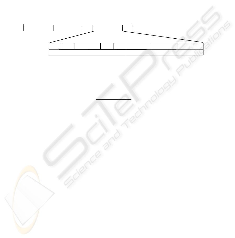
algorithms is applied. Chromosomes are generated for every individual from the

initial population as follows, see Fig. 1:

individual 1

individual 2

...

individual k

...

. . .

h+1

. . .

h+o

h+0

units in the hidden layer

units in the output layer

Fig. 1. Population of individuals and their chromosomes.

Symbols b

(i = 1, …,h+o) refers to varies types of activation functions [10]:

− b

= 1, if the activation function is a binary sigmoid function:

()

−+

exp1

(1)

where

is the steepness parameter, which value is set in the initial population

randomly (e.g.

∈ (0; 7>).

− b

= 2, if the activation function is a binary step function with threshold

()

⎩

⎨

⎧

≥

xif

(2)

the steepness parameter

is not define here thus we assigned value 0 to it.

− b

= 3 if the activation function is a Gaussian function:

(

)

(

)

exp xxf −= .

(3)

the steepness parameter

is not define here thus we assigned value 0 to it.

− b

= 4, if the activation function is a saturated linear function:

()

⎪

⎩

⎪

⎨

⎧

≤≤

xif

xifx

xif

(4)

the steepness parameter

is not define here thus we assigned value 0 to it.

Next, we calculate an error value (E) between the desired and the real output after

defined partial training with genetic algorithms. Adaptation of each individual starts

with randomly generated weight values that are the same for each neural network in

the given population. On the basis of it is calculated a fitness function for every

individual as follows:

Fitness

= E

max

- E

. (5)

for i = 1, ...,N,

where E

is error for the i-th network after a partial adaptation;

max

is a maximal error for the given task,

max

= o

pattern

(o is number of output units and pattern is number of patterns);

N is the number of individuals in the population.

All of the calculated fitness function values of the two consecutive generations are

sorted descending and the neural network representation attached to the first half

creates the new generation. For each fitness function is calculated the probability of

reproduction its existing individual by standard method [11]. One-point crossover was

used to generate two offspring. If the input condition of mutation is fulfilled (e.g. if a

randomly number is generated, that is equal to the defined constant), one of the

individual is randomly chosen. There is randomly replaced one place in its genetic

representation by a random value from the set of permitted values. Our calculation

finishes, when the population is composed only from the same individuals.

4 Experiments

In order to test the efficiency of described method, we applied it to the alphabet

coding problem that exists in cryptography. Neural networks can be also used in

encryption or decryption algorithms, where parameters of adapted neural networks are

included to cipher keys [12]. Cipher keys must have several heavy attributes. The best

one is the singularity of encryption and cryptanalysis [13]. Encryption is a process in

which we transform the open text (e.g. news) to cipher text according to rules.

Cryptanalysis of the news is the inverse process, in which the receiver of the cipher

transforms it to the original text. The open text is composed from alphabet characters,

digits and punctuation marks. The cipher text has usually the same composition as the

open text.

We worked with multilayer neural networks, which topologies were based on the

training set (see Table 1). The chain of chars of the plain text in a training set is

equivalent to a binary value that is 96 less than its ASCII code. The cipher text is then

a random chain of bits.

Table 1. The set of patterns (the training set).

THE PLAIN TEXT

THE

CIPHER

TEXT

THE PLAIN TEXT

THE

CIPHER

TEXT

Char ASCII

code

(DEC)

The

chain

of bits

The chain

of bits

Char ASCII

code

(DEC)

The

chain

of bits

The

chain

of bits

a 97 00001 000010 n 110 01110 011100

b 982 00010 100110 o 111 01111 101000

c 99 00011 001011 p 112 10000 001010

d 100 00100 011010 q 113 10001 010011

e 101 00101 100000 r 114 10010 010111

f 102 00110 001110 s 115 10011 100111

g 103 00111 100101 t 116 10100 001111

h 104 01000 010010 u 117 10101 010100

i 105 01001 001000 v 118 10110 001100

j 106 01010 011110 w 119 10111 100100

k 107 01011 001001 x 120 11000 011011

l 108 01100 010110 y 121 11001 010001

m 109 01101 011000 z 122 11010 001101

The initial population contains 30 three-layer feedforward neural networks. Each

network architecture is 5 - 5 - 6 (e.g. five units in the input layer, five units in the

hidden layer, and six units in the output layer), because the alphabet coding problem

is not linearly separable and therefore we cannot use neural network without hidden

units. The nets are fully connected. We use the genetic algorithm with the following

parameters: probability of mutation is 0.01 and probability of crossover is 0.5.

Adaptation of each neural network in given population starts with randomly generated

weight values that are the same for each neural network in the population. We also

used genetic algorithms with the same parameters for the partial neural network

adaptation, where number of generations for a partial adaptation was 500. Its

chromosome representation is described in [14].

History of the error function is shown in the figure 3. There are shown average

values of error functions in the given population. Other numerical simulations give

very similar results. The “binary sigmoid function” represents an average value after

adaptation with the binary sigmoid activation function consecutively with all

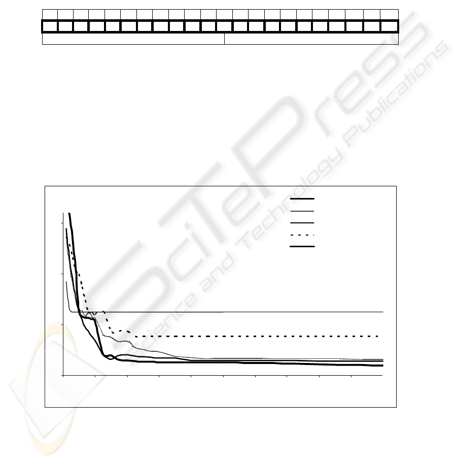
steepness parameters

= {1,2,3,4,5,6,7}. The “binary step function” represents an

adaptation with the binary step activation function (with the threshold

), the

“saturated linear function” represents an adaptation with the saturated linear

activation function, and “Gaussian activation” represents an adaptation with the

Gaussian activation function. Each of these mentioned representations is associated

with all units in given neural network architecture. Opposite of this, the “best

individual” represents an adaptation of the best individual in population, which

chromosome is the following, see Fig. 2:

1 5 1 7 1 1 3 0 1 5 3 0 1 7 3 0 1 5 1 6 1 2

units in the hidden layer units in the output layer

Fig. 2. The “best individual” chromosome in the last population.

5 Conclusions

All networks solve the alphabet coding task in our experiment, but artificial neural

network with evolving transfer functions of each unit works well, because several

different types of neurons are usually necessary to solve a problem. We can see that

the proposed technique is really efficient for the presented purpose, see the Fig. 3.

Networks with too many copies of the same neuron work usually worse.

0 100 200 300 400 500 600 700 800 900

number of generati on

binary sigmoid f unction

Gauss f unction

binary step f unction

saturated linear function

best individual

Fig. 3. The error function history.

Here, the transfer function is shown to be an important part of architecture of the

artificial neural network and have significant impact on artificial neural network’s

performance. Transfer functions of different units can be different and decided

automatically by an evolutionary process, instead of assigned by human experts. In

general, nodes within a group, like layer, in an artificial neural network tend to have

the same type of transfer function with possible difference in some parameters, while

different groups of nodes might have different types of transfer function.

References

1. Liu, Y. and Yao, X. “Evolutionary design of artificial neural networks with different

nodes”. In Proc. 1996 IEEE Int. Conf. Evolutionary Computation (ICEC’96), Nagoya,

Japan, pp. 670–675.

2. Fogel, D. B., Evolutionary Computation: Toward a New Philosophy of Machine

Intelligence. New York: IEEE Press, 1995.

3. Bäck, T. Hammel, U.and Schwefel, H.-P.“Evolutionary computation: Comments on the

history and current state,” IEEE Trans. Evolutionary Computation, vol. 1, pp. 3–17, Apr.

1997.

4. Mani, G. “Learning by gradient descent in function space”. In Proc. IEEE Int. Conf.

System, Man, and Cybernetics, Los Angeles, CA, 1990, pp. 242–247.

5. Lovell D. R. and Tsoi, A. C. The Performance of the Neocognitron with Various S-Cell and

C-Cell Transfer Functions, Intell. Machines Lab., Dep. Elect. Eng., Univ. Queensland,

Tech. Rep., Apr. 1992.

6. Stork, D. G. Walker, S. Burns, M. and Jackson, B. “Preadaptation in neural circuits”. In

Proc. Int. Joint Conf. Neural Networks, vol. I, Washington, DC, 1990, pp. 202–205.

7. White D. and Ligomenides, P. “GANNet: A genetic algorithm for optimizing topology and

weights in neural network design”. In Proc. Int. Workshop Artificial Neural Networks

(IWANN’93), Lecture Notes in Computer Science, vol. 686. Berlin, Germany: Springer-

Verlag, 1993, pp. 322–327.

8. Hwang, M. W. Choi, J. Y. and Park, J. “Evolutionary projection neural networks”. In Proc.

1997 IEEE Int. Conf. Evolutionary Computation, ICEC’97, pp. 667–671.

9. Sebald, A. V. and Chellapilla, K. “On making problems evolutionarily friendly, part I:

Evolving the most convenient representations”. In Porto, V. W., Saravanan, N., Waagen, D.

and Eiben, A. E. (Eds.): Evolutionary Programming VII: Proc. 7th Annu Conf.

Evolutionary Programming, vol. 1447 of Lecture Notes in Computer Science, Berlin,

Germany: Springer-Verlag, 1998, pp. 271–280.

10. Volná E. “Evolution design of an artificial neural network with fixed topology”, In R.

Matoušek, P. Ošmera (eds.): Proceedings of the 12th International Conference on Soft

Computing, Mendel'06, Brno, Czech Republic, 2006, pp. 1-6.

11. Lawrence, D. Handbook of genetic algorithms. Van Nostrand Reinhold, New York 1991.

12. Volná, E. „Using Neural network in cryptography“. In P. Sinčák, J. Vaščák, V. Kvasnička,

R. Mesiar (eds.): The State of the Art in Computational Intelligence. Physica-Verlag

Heidelberg 2000. pp.262-267.

13.

Garfinger, S. PGP: Pretty Good Privanci. Computer Press, Praha 1998.

14. Volná, E. „Learning algorithm which learns both architectures and weights of feedforward

neural networks“. Neural Network World. Int. Journal on Neural & Mass-Parallel Comp.

and Inf. Systems. 8 (6): 653-664, 1998.