
ON TUNING THE DESIGN OF AN EVOLUTIONARY ALGORITHM
FOR MACHINING OPTIMIZATION PROBLEMS
Jean-Louis Vigouroux
1,2
, Sebti Foufou
1
, Laurent Deshayes
3
James J. Filliben
4
, Lawrence A. Welsch
5
and M. Alkan Donmez
5
1
Laboratoire Electronique, Informatique et Image (Le2i), University of Burgundy, Dijon, France
2
Currently a guest researcher at the National Institute of Standards and Technology (NIST), Gaithersburg, MD, USA
3
Laboratoire de M
´
ecanique et Ing
´
enieries, IFMA and University of Auvergne, Clermont-Ferrand, France
4
Information Technology Laboratory, at NIST, Gaithersburg, MD, USA
5
Manufacturing Engineering Laboratory, at NIST, Gaithersburg, MD, USA
Keywords:
Evolutionary algorithms, Experimental Algorithmics, Optimization of machining parameters.
Abstract:
In this paper, a novel method for tuning the design of an evolutionary algorithm (EA) is presented. The
ADT method was built from a practical point of view, for including an EA into a framework for optimizing
machining processes under uncertainties. The optimization problem studied, the algorithm, and the computer
experiments made using the ADT method are presented with many details, in order to enable the comparison
of this method with actual methods available to tune the desing of evolutionary algorithms.
1 INTRODUCTION
A mathematical framework for optimizing machining
processes with uncertainties, called the Robust Opti-
mizer, is currently being developed at the National In-
stitute of Standards and Technology (NIST), as a part
of the Smart Machining Systems Research Program
(Deshayes et al., 2005b). The goal of this frame-
work is to provide a process optimization capabil-
ity for machine-tools, integrated with the CAD/CAM
systems and the machine-tool controllers. Optimiza-
tion of machining processes is a difficult task which
has been studied since the beginning of the last cen-
tury. As an example, the selection of optimal cut-
ting parameters involves the development of machin-
ing models, and optimization algorithms able to han-
dle those models. Taylor built the first experimental
models in a seminal study (Taylor, 1907); after him
many different models and optimization algorithms
were developed. The class of optimization problems
encountered can be linear, convex non-linear, or non-
convex as shown by Deshayes et al. (Deshayes et al.,
2005a). For example in high-speed machining pro-
cesses, the constraint for chatter stability is defined
by a non-convex function. Additionally, as shown
by Kurdi et al. (Kurdi et al., 2005), uncertainties
on model parameters may strongly influence the limit
contours of the constraint. As a consequence, the
framework under development must contain several
algorithms for optimization under uncertainties such
as robust linear programming, stochastic program-
ming, depending on the class of optimization prob-
lems. Vigouroux et al. (Vigouroux et al., 2007) pre-
sented a novel optimization algorithm to fit into the
framework, for non-convex problems, by coupling an
evolutionary algorithm with interval analysis. EA are
algorithms from the Artificial Intelligence domain.
The main mechanism of EA is an iterative sampling
of candidate solutions to find the optimal one, for
more information see the book of Yao (Yao, 1999).
The latest applications of EA include Pattern recog-
nition (Raymer et al., 2000), multi-disciplinary opti-
mization for car design (Rudenko et al., 2002). EA
have already been applied in machining by Wang et
al. (Wang et al., 2002) to a non-convex optimization
problem without uncertainties. EA are algorithms that
require tuning of their parameters to obtain optimal
results regarding execution time, convergence, and
accuracy. Moreover the parameters must be robust
for a range of similar problems.
The design of evolutionary algorithms, that is the
choice of an EA architecture and algorithm parame-
ters, robust to problem parameter changes, or adapted
to several problems is not straightforward. There-
240
Vigouroux J., Foufou S., Deshayes L., J. Filliben J., A. Welsch L. and Alkan Donmez M. (2007).
ON TUNING THE DESIGN OF AN EVOLUTIONARY ALGORITHM FOR MACHINING OPTIMIZATION PROBLEMS.
In Proceedings of the Fourth International Conference on Informatics in Control, Automation and Robotics, pages 240-247
DOI: 10.5220/0001624802400247
Copyright
c
SciTePress

fore, evolutionary algorithms have found applications
in specific optimization problems where the tuning of
the algorithm can be performed by the user. Several
methods to help this design were introduced recently
by Francois and Lavergne (Francois and Lavergne,
2001), Nannen and Eiben (Nannen and Eiben, 2006).
Nannen and Eiben were interested to design an evolu-
tionary system to study evolutionary economics. For
that complex system, EA are not just an optimization
algorithm but also a model for simulating evolution.
Therefore the EA used by Nannen and Eiben contain
much more parameters than the EA studied here: over
ten. Nannen and Eiben don’t have an alternate method
at hand to find the optimum solution, mainly because
the EA studied does not perform optimization. To op-
timize the parameters of the EA, they built the CRE
method, by considering a trade-off between a per-
formance index,the average response of the EA, and
the average algorithm complexity, for 150 samples of
the algorithm parameters. To take in account simi-
lar problems, they let vary three problem parameters
and do 18 experiments. For each of them, an iterative
routine determines automatically the optimal values
of the algorithm parameters, based on the trade-off.
Then the optimal values of the parameters are found
as the average over all experiments.
The relevance of such methods is important to in-
tegrate EA in the Robust Optimizer. Machining prob-
lems have many parameters subject to changes. In
this paper, an alternative method to the CRE method,
the algorithm design tuning (ADT) method, is pre-
sented for helping the design of an EA for machin-
ing optimization problems. It makes use of statisti-
cal engineering tools not only to optimize the algo-
rithm parameters, but to modify the EA design in or-
der to avoid non-convergence. In the background of
the study are presented the example turning problem
used for building the Robust Optimizer, along with
the EA able to solve it, and some notions about ex-
perimenting with algorithms. Then the novel ADT
method is introduced along with experimental results
and a comparison with the CRE method.
2 BACKGROUND
2.1 Example Turning Problem for the
Robust Optimizer
An optimization problem consists of optimizing
an objective function while satisfying several con-
straints:
Minimize f(x)
subject to g
j
(x) ≤ 0 j = 1,2... p
where f is the objective function, g
j
a constraint func-
tion, and x is a vector of real variables, called a so-
lution of the problem. The vectors x
l
and x
u
define
the lower and upper bounds for the variables, and
are specified in some of the constraint equations g
j
.
These bounds define the search space.
The turning problem is a two-variable optim
ization problem, with a set of specific values for the
problem parameters. The variables and parameters
used in the problem are presented below:
f- Feed, mm/rev
Vc- Cutting speed, m/s
a
p
- Depth of cut, mm
f
min
- Minimum Feed, mm/rev
f
max
- Maximum Feed, mm/rev
Vc
min
- Minimum Cutting speed, m/s
Vc
max
- Maximum Cutting speed, m/s
Pu- Spindle power, W
Cu- Spindle torque, N ˙m
Ra
spe
- Workpiece desired surface roughness, µm
Ra- Workpiece surface roughness, µm
K
1
,δr
epsilon
- Constants in surface roughness equation
r
epsilon
- Tool nose radius, mm
F
c
- Cutting force, N
K
c
- Constant in cutting force equation
tc- Exponent in cutting force equation
T- Tool life, s
T
r
,f
r
,a
pr
,Vc
r
- Constants in tool life equation
n,m,l- Exponents in tool life equation
t
cut
- Cutting time, s
N
parts
- Desired number of parts to cut per tool
A- Workpiece equivalent cutting surface, mm
2
D
av
- Workpiece average diameter, mm
L
c
- Workpiece equivalent length of cut, mm
The goal is to find the optimal machining param-
eters, feed and speed, which maximize the material
removal rate (MRR) of one turning pass, considering
several process constraints. The two variables to be
optimized are the feed f and the cutting speed Vc.
The mathematical functions of the problem are de-
tailed below:
The objective function is defined as the opposite of
MRR in order to solve a minimization problem
1
:
f( f,Vc) = −ap× f ×Vc (1)
The constraint function of minimum feed, C1:
g
1
( f,Vc) = f
min
− f (2)
The constraint function of maximum feed, C2:
g
2
( f,Vc) = f − f
max
(3)
1
To maximize an objective function is the same as to
minimize its negative opposite.
ON TUNING THE DESIGN OF AN EVOLUTIONARY ALGORITHM FOR MACHINING OPTIMIZATION
PROBLEMS
241

The constraint function of minimum cutting speed,
C3:
g
3
( f,Vc) = Vc
min
−Vc (4)
The constraint function of maximum cutting speed,
C4:
g
4
( f,Vc) = V
c
−Vc
max
(5)
The constraint function of surface roughness, C5:
g
5
( f,Vc) = Ra( f) − Ra
spe
(6)
The constraint function of tool life, C6:
g
6
( f,Vc) = T( f,Vc) − t
cut
( f,Vc) (7)
The constraint function of Spidle power life, C7:
g
7
( f,Vc) = Pu− F
c
( f,Vc) ×V
c
(8)
Several functions have variables defined by the equa-
tions presented below. The tool life equation is ob-
tained from Taylor’s work (Taylor, 1907):
T( f,Vc) = T
r
a
p
a
pr
l
f
f
r
m
.
V
c
V
cr
n
(9)
The cutting time, t
cut
, is obtained from the following
equation:
t
cut
( f,Vc) = N
parts
A
f × V
c
× 1000
, (10)
where A is obtained from the following equation:
A = π× D
av
× L
c
. (11)
The surface roughness equation is obtained from the
study by Deshayes et al. (Deshayes et al., 2005a):
Ra( f) = K
1
f
δr
epsilon
r
epsilon
. (12)
The cutting force equation is obtained from an exper-
imental study by Ivester et al. (Ivester et al., 2006):
Fc( f) = Kc× f
1+tc
× ap. (13)
The original problem has parameter values given
in Table (1). For this original problem, the limit con-
tours of the constraint functions are represented in
Figure (1). Ten parameters of this problem can be
modified and are specified in Table (1). The parame-
ter ranges of this table are determined by knowledge
of machining and judgement.
2.2 Evolutionary Algorithms
In Darwin’s evolution theory (Darwin, 1859), a popu-
lation of individuals evolves over several generations.
The individuals with the best fitness, determined by
their genes, are selected to breed; their children form
the next population. Since offspring of individuals
Table 1: Problem parameter ranges.
Parameter Original Minimum Maximum Factor
name value value value name
Vc
min
1.83 1.33 2.5 X1
Vc
max
7.5 6.5 10 X2
f
min
0.2 0.1 0.3 X3
f
max
0.6 0.5 0.8 X4
a
p
2 1 4 X5
K
c
2000 1800 2500 X6
Pu 15000 15000 20000 X7
D
av
72 60 80 X8
L
c
550 350 650 X9
Ra
spe
4.5 3 5 X10
with best fitness should be better suited to survive
within their environment, the species improves. Thus,
over time and several generations, evolution leads to
the adaptation of the population to the environment.
This theory is used by the implemented Evolution-
ary Algorithm (EA). The optimization variables play
the role of the individuals’ genes. The EA is presented
as a class written in the Python language
2
. The con-
structor function of this class is presented below:
class EA:
def __init__(self):
self.gene_size=2
x1bounds=[0.2,0.6]
x2bounds=[1.83,7.5]
self.bounds = [x1bounds,x2bounds]
self.N = 50
self.alpha=0.4
self.z=20
The constructor sets the number of genes per individ-
ual (here two), the bounds of variables, the population
size N, the breeding parameter α, and the number of
generations z. The
run_algorithm
function contains
the algorithm steps and is presented here:
def run_algorithm():
population = population_initialize()
for i in range(self.z):
parent_population =
tournament_selection(population)
children_population =
breeding(parent_population)
population = children_population
return population[1]
2
Certain trade names and company products are men-
tioned in the text or identified in an illustration in order to
adequately specify the experimental procedure and equip-
ment used. In no case does such an identification imply rec-
ommendation or endorsement by the National Institute of
Standards and Technology, nor does it imply that the prod-
ucts are necessarily the best available for the purpose. Offi-
cial contribution of the National Institute of Standards and
Technology; not subject to copyright in the United States.
ICINCO 2007 - International Conference on Informatics in Control, Automation and Robotics
242

The EA has the following steps:
• Construction of the initial population. The
population_initialize
function, presented
below, outputs a first population of N individuals
spread uniformly over the search space, by use of
a
random
function giving a number between zero
and one. The fitness function, h, of one individ-
ual is computed with the static penalty method,
and is given in Equation (14). Michalewicz et al.
(Michalewicz et al., 1996) reviewed several meth-
ods that enable EA to handle optimization prob-
lems with constraints, and explain this method
with more details.
def population_initialize():
population = []
for i in range(self.pop_size):
population.append([])
for j in range(self.gene_size):
population[i].append(self.bounds[j][0]+
(self.bounds[j][1]
- self.bounds[j][0])*random())
population[i].append(fitness(population[i]))
return population
def fitness(genes):
result=h(genes)
return result
h(x) = −sf(x) +W ×
n
∑
j=1
sg
j
(x) (14)
with
sf(x) =
f(x)
f(x
u
)
(15)
and
sg
j
(x) =
g
j
(x)
g
j
(x
u
)
if g
j
(x) ≤ 0, 0 else
(16)
W is the static penalty parameter. This parame-
ter controls the degradation of the fitness function
when one or more constraints are violated. In this
article, the value of W is ten.
• Selection. The
tournament_selection
func-
tion, presented below, outputs a parent population
of N/2 individuals. These individuals are selected
by N/2 tournaments of size 2: for each tournament
two individuals are randomly picked in the pop-
ulation and their fitness functions are compared.
The individual with the higher fitness value wins
and is added to the parent population. The loser
re-enters the population and can eventually par-
ticipate in another tournament.
def tournament_selection(population):
pool_size=self.N/2
parent_population = []
for i in range(pool_size):
parent_population.append([])
match = Structure()
match.pool = sample(population,2)
match.knight1=match.pool[0]
match.knight2=match.pool[1]
if match.knight1[2] <match.knight2[2]:
match.winner = match.knight1
elif match.knight1[2] ==match.knight2[2]:
match.winner = match.knight1
else:
match.winner = match.knight2
parent_population[i] = match.winner
return parent_population
• Breeding. The
breeding
function, presented be-
low, outputs a new children population. Two indi-
viduals are randomly picked from the parent pop-
ulation. Two new individuals are created in a box.
The position of this box within the search space
is defined by the two parents’ genes. The dimen-
sions of the box are defined by both a breeding pa-
rameter called α and the two parents’ genes. This
process of creating individuals is called blend
crossover and was introduced by Eschelman and
Schaffer (Eschelman and Schaffer, 1993). It is re-
peated N/2 times in order to produce a children
population having N individuals.
def breeding(parent_population):
children_population = []
for i in range(self.pool_size):
parents = sample(parent_population,2)
parent1 = parents[0]
parent2 = parents[1]
children1 = []
children2 = []
for j in range(self.gene_size):
a= -self.alpha +(1+2*self.alpha)*random()
children1.append(a*parent1[j] +
(1-a)*parent2[j])
a= -self.alpha +(1+2*self.alpha)*random()
children2.append(a*parent1[j] +
(1-a)*parent2[j])
children1.append(fitness(children1))
children2.append(fitness(children2))
children_population.append(children1)
children_population.append(children2)
return children_population
At the next generation, this new population will
face again the selection step and the loop will con-
tinue until the number of generations z, is attained.
When the algorithm is stopped, the first individual in
the population, with genes (x
11
,x
21
), is picked. The
objective function MRR
z
is computed for this individ-
ual in Equation (17) and is the result output by the
algorithm.
MRR
z
= a
p
× x
11
× x
21
(17)
For the original problem, the populations at several
generations are plotted in Figure (1). The initial pop-
ulation is represented by stars, the population at gen-
eration 2 is represented by circles, and the popula-
tion at generation 5 is represented by diamonds. The
ON TUNING THE DESIGN OF AN EVOLUTIONARY ALGORITHM FOR MACHINING OPTIMIZATION
PROBLEMS
243
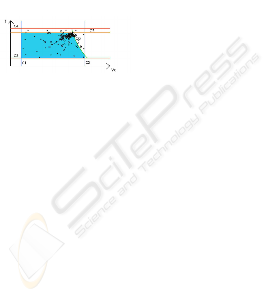
evolution of the center of gravity of the population
over several generations defines a track represented
by crosses and dashed lines. This algorithm has three
influential parameters: the breeding parameter α, the
population size N, and the number of generations, z.
Tuning of these parameters is required to enhance the
performance of the algorithm.
Figure 1: Populations at several generations during one run
of the EA.
2.3 Experimental Algorithmics
Experimental Algorithmics refer to the study of al-
gorithms through a combination of experiments and
classical analysis and design techniques.
Since EA are randomized algorithms, their results
are unequal run after run, even though all parameters
may remain the same. Therefore, it is necessary to run
the EA several times to report an average result. Thus,
the computational expense associated with the tun-
ing of the algorithm may become important. Statis-
tical techniques such as design of experiments and re-
sponse surface methodology avoid this computational
expense and are presented in (NIST/SEMATECH,
2006) and (Box et al., 1978).
A computer experiment refers here to a run of the
EA with a set of algorithm parameters and a set of
problem parameters. With the design of experiments,
the problem parameters are renamed factors, see
Table (1); a design stands for a set of experiments,
with each experiment having a specific combination
of factor levels. When considering only two levels
of variation for each problem parameter, the low
settings and the high settings presented in Table
(1), there are 1024 possible combinations. A full
factorial design is a set with all possible factor levels
combinations, here 2
10
= 1024. A more efficient
design is an orthogonal fractional factorial design
(NIST/SEMATECH, 2006), with only 128 runs, ten
percent of the full factorial design.
According to the response surface terminology
(Box et al., 1978), the measures made during the ex-
periments are referred to as response variables.
For the design of the EA, three response variables
are considered:
• y
1
is an index defining the accuracy of the EA:
y
1
=
MRR
z
MRR
∗
(18)
where MRR
∗
is the optimal material removal rate
of the problem, corresponding to the optimal so-
lution. MRR
∗
can be obtained graphically or
by another optimization algorithm able to find
it. Since MRR is an increasing function, The ex-
pected range of y
1
is between 0 and 1. If the value
of y
1
is greater, the result MRR
z
output by the al-
gorithm is unacceptable and it means that the al-
gorithm did not converge.
• y
2
is the count of non-convergence cases af-
ter several runs of the algorithm. Those non-
convergence cases are detected by values of y
1
higher than 1.
• y
3
is a time measure in seconds, related to the ex-
ecution time of the EA.
The set-up of the computer experiments is given:
The EA is implemented with Matlab software on a
personal computer. The computer processor is an In-
tel Pentium 4 with a frequency of 3.80 GHz, running
with a memory of size 2 GB. The measure of y
3
is
made using Matlab’s cputime function.
The random function used to generate the neces-
sary random behaviors in the algorithm is Matlab’s
random function with the Seed method. It gener-
ates a pseudo-random number between 0 and 1. Af-
ter a certain number of calls, 2
31
− 1, the function
repeats itself. This function takes as the argument a
number called the seed. The seed defines the internal
state of the function and, with the same seed, the ran-
dom function generates the same sequence of random
numbers. Therefore, all the seeds used in the experi-
ments were recorded and stored, giving the possibility
to reproduce exactly the same experimental results.
Each computer experiment was replicated ten times
with different seeds.
Once the computer experiments have been made,
the Exploratory Data Analysis (EDA) techniques
(Tukey, 1977) can be used to explore the results.
These techniques allow to ferret out interesting at-
tributes of the result data. The Dataplot statistical en-
gineering software was used in this study to perform
EDA. Sensitivity analysis is a technique that allows to
order the problem parameters according to the effect
of their variation on the response. The order of the
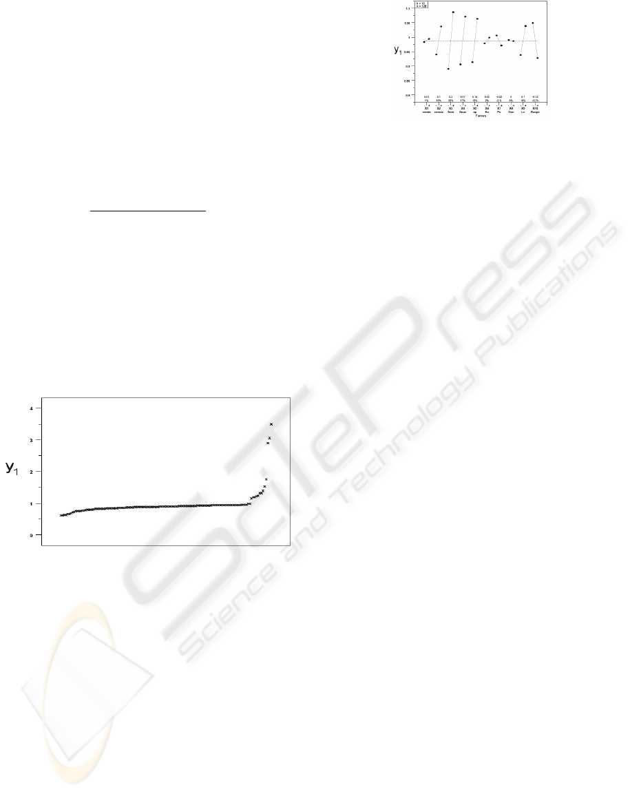
parameter can be deduced from a plot called the main
effect plot. An example plot is shown in Figure (3).
ICINCO 2007 - International Conference on Informatics in Control, Automation and Robotics
244
3 THE ADT METHOD
3.1 Step 1: Preliminary Exploratory
Data Analysis
The first step of the methodology is to perform an
exploratory analysis. The goal is to see how much
the algorithm performances vary, and to establish if
the algorithm needs any modifications of its architec-
ture. This analysis requires performing computer ex-
periments with a set of algorithm parameters (α,N,z),
according to the orthogonal fractional
factorial design
introduced previously. This step requires a special
plot of the response y
1
: the responses of all exper-
iments are ordered and plotted, as shown in Figure
(2). The experiments where the algorithm does not
converge are detected by values of y
1
exceeding one.
The reason for non-convergence can be discovered by
plotting the limit contours of the constraints for the
case with non convergence, similarly to Figure (1)
presented previously. Then the algorithm architecture
may be modified, in order to be adapted to the non-
convergence cases.
Figure 2: Ordered data plot of response y
1
for the ex-
ploratory analysis of the set (α = 0.4, N = 40,z = 20).
3.2 Step 2: Sensitivity Analysis
This step is optional. This step may only be re-
quired if the problem has more than two optimiza-
tion variables, where it may be impossible to plot
the limit contours of the constraints for the case with
non-convergence. In that case the reason for non-
convergence cannot be easily discovered. The sen-
sitivity analysis allows to determine the most impor-
tant problem parameters affecting the response y
1
.
The main effect plot in Figure (3) shows the varia-
tion of the response y
1
depending on the variation of
the problem parameters.
Figure 3: Main effect plot of response y
1
for the sensitivity
analysis of the set (α = 0.4, N = 40,z = 20).
3.3 Step 3: Optimization
In this step the algorithm parameters are
optimized(α,N,z). α,N,z can be chosen respec-
tively in the range [20, 200],[0.1, 0.9] and [10,
50]. Given a set (α,N,z), a sensitivity analysis is
performed as previously discussed, but the results of
each computer experiment are now three responses,
y
1
, y
2
, and y
3
. The goal is to optimize the average
values of the responses: maximize ¯y
1
, minimize ¯y
2
,
minimize ¯y
3
.
First, only the first objective ¯y
1
is considered.
Since the computational expense of the sensitivity
analysis necessary to compute ¯y
1
is high, only a small
number of sets (α,N,z) can be investigated. The re-
sponse surface methodology is applied to find the best
set (α,N,z). Starting with an initial guess (α
0
,N
0
,z
0
),
several other sets in the neighborhood are tested,
whose values are defined by an orthogonal full fac-
torial design. This design has 3 factors and 11 exper-
iments. The choice of the parameter ranges, centered
around the set (α
0
,N
0
,z
0
), is left to the user.
The result ¯y
1
of each tested set (α,N,z) can be vi-
sualized as a cube, as shown in Figure (4). From the
analysis of the cube, a new center set (α
1
,N
1
,z
1
) is
chosen, to explore the space in the region where the
optimum value of ¯y
1
, ¯y
1
∗
, could be located. Again,
computer experiments are performed with the same
design but with different parameter ranges, in order
to acquire the new cube with center (α
1
,N
1
,z
1
). This
iterative process can be repeated as long as needed in
order to find ¯y
1
∗
. The cubes for the objectives ¯y
2
and
¯y
3
can be acquired at the same time, although the op-
timum values for these objectives are not found. This
method enables one to explore the spaces ¯y
2
and ¯y
3
as
functions of variables (α,N,z). After the three objec-
tive spaces have been explored, the user is able to pick
a set (α,N,z), that has good values ¯y
1
, ¯y
2
, and ¯y
3
, al-
though not optimal. This set represents a compromise
between best accuracy, best convergence, and best ex-
ecution time.
ON TUNING THE DESIGN OF AN EVOLUTIONARY ALGORITHM FOR MACHINING OPTIMIZATION
PROBLEMS
245
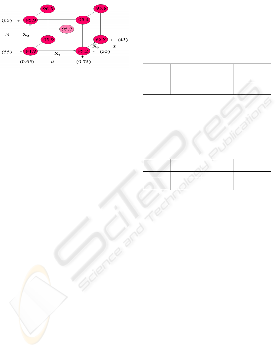
Figure 4: The responses ¯y
1
multiplied by 100 for the cube
with center (α
0
= 0.7, N
0
= 60, z
0
= 40).
3.4 Validation of the Optimized
Algorithm
The algorithm is optimized with a sample of prob-
lem parameter combinations and a sample of seeds.
This sample can be termed a training data set, and an
analogy can be drawn with the training of neural net-
works. Now the performance results of the algorithm
must be verified with a new sample of data: the vali-
dation data set.
In order to compare the average performance re-
sults, a validation data set of the same size as the train-
ing data set must be chosen. A different sampling of
the problem parameter combinations is made. A Latin
hypercube sampling is used with the same size as the
orthogonal design presented in Section (2.3): 128 val-
ues for each of the ten factors. A new sample of 100
different seeds is also picked and stored. The sensitiv-
ity analysis can be replicated ten times with the new
data and the results compared.
3.5 Results
The preliminary exploratory analysis was performed
on the set (α = 0.4, N = 40, z = 20). The ordered data
plot of response y
1
, shown in Figure (2), revealed non-
convergence cases, detected on the right of the plot by
values exceeding one. The limit contours of the con-
straints were plotted for some of the non-convergence
cases, and it was discovered that the initialization step
was not adapted. To avoid this problem, it was de-
cided to change the initialization so that the first pop-
ulation is spread in the lower left quarter of the search
space. The sensitivity analysis, shown in Figure (3),
was performed, but all the information provided by
this step was already known from the plots of the first
step.
In the third step, optimization was performed with
an initial guess (α
0
= 0.7, N
0
= 60, z
0
= 40). Af-
ter three iterations, it was found that ¯y
1
∗
should have
a value around 0.97, and a good confidence was ac-
quired about the knowledge of the three objective
spaces. The set of algorithm parameters selected is
(α = 0.6, N = 60, z = 40). The results of a sensitiv-
ity analysis of this set, replicated ten times, is shown
in Table (2). During the validation step, a compari-
Table 2: Optimization step: results for the set (α = 0.6,N =
60,z = 40) with the training data set.
Response Response Response
variable ¯y
1
variable ¯y
2
variable ¯y
3
(s)
average 0.950 1 1.130
standard 0.002 1.05 0.003
deviation
son was made between the results obtained with the
training data set and the results obtained with the val-
idation data set. The later results presented in Table
(3) are slightly better. Therefore, the training method
used to tune the algorithm seems to be sound.
Table 3: Validation step: results for the set (α = 0.6,N =
60,z = 40) with the validation data set.
Response Response Response
variable ¯y
1
variable ¯y
2
variable ¯y
3
(s)
average 0.966 0 1.123
standard 0.001 0.00 0.002
deviation
3.6 Comparison with the Cre Method
The ADT method was developped for the turning
problem of the Robust Optimizer. From this point of
view the EA has few parameters, three, and quite a lot
of problem parameters, ten. On the contrary, the CRE
method considers many EA parameters and few prob-
lem parameters. The reason why the CRE method
does not consider many problem parameters may be a
reason of time consumed to perform the experiments,
as indicated in the paper by Nannen and Eiben (Nan-
nen and Eiben, 2006). The ADT method required also
a lot of time to perform the experiments. For both
methods, increasing the number of algorithm param-
eters and problem parameters considered is a prob-
lem, so the complexity of the CRE and ADT methods
should be determined and compared.
The CRE method relies on information theory to
determine the importance of the algorithm parame-
ters. This point is not adressed by the ADT method.
During the study, it was decided to remove the muta-
tion parameter from the algorithm by studying videos
showing the populations evolve over the search space,
during several iterations. This kind of decision was
made possible because of the low dimension of the
optimization problem studied: only two variables.
ICINCO 2007 - International Conference on Informatics in Control, Automation and Robotics
246

The ADT method enables to optimize very practi-
cal responses of EA: the execution time, the number
of non-convergence cases, the accuracy. For the last
objective, accuracy, one needs to know the optimal
solution for each optimization problem. This is possi-
ble graphically only for low dimension optimization
problems. For optimization problems of higher di-
mension, an alternative optimization algorithm must
be used.
Since this method was developped concurrently
with the CRE method, an experimental comparison
of the two methods was not possible. However all de-
tails are given in this paper to perform such a study.
4 CONCLUSION
The novel ADT method presented here enables tun-
ing the design of an EA for optimizing a turning pro-
cess with uncertainties. The ADT method also en-
ables the algorithm designer to manage several per-
formance objectives. The method is an alternative
method to the CRE method, and focuses on the practi-
cal objectives of accuracy, non-convergence and exe-
cution time. In the future, the two methods need to be
compared. For the Robust Optimizer, an optimization
problem involving a milling process needs to be con-
sidered, to see if the ADT method enables to design an
EA for optimizing different kinds of machining pro-
cesses, or not.
ACKNOWLEDGEMENTS
The authors would like to acknowledge the support
and assistance of Robert Ivester, David Gilsinn, Flo-
rian Potra, Shawn Moylan, and Robert Polvani, from
the National Institute of Standards and Technology.
REFERENCES
Box, G. E. P., Hunter, W. G., and Hunter, J. S. (1978).
Statistics for Experimenters. John Wiley.
Darwin, C. (1859). On the origin of species by means of
natural selection. John Murray.
Deshayes, L., Welsch, L., Donmez, A., and Ivester, R. W.
(2005a). Robust optimization for smart machining
systems: an enabler for agile manufacturing. In Pro-
ceedings of IMECE2005: 2005 ASME International
Mechanical Engineering Congress & Exposition.
Deshayes, L., Welsch, L., Donmez, A., Ivester, R. W.,
Gilsinn, D., Rohrer, R., Whitenton, E., and Potra, F.
(April 3-5, 2005b). Smart machining systems: Issues
and research trends. In Proceedings of the 12th CIRP
Life Cycle Engineering Seminar.
Eschelman, L. and Schaffer, J. D. (1993). Real-coded
genetic algorithms and interval-schemata. Morgan
Kaufmann.
Francois, O. and Lavergne, C. (2001). Design of evolution-
ary algorithms-a statistical perspective. IEEE Trans-
actions on Evolutionary Computation, 5(2):129–148.
Ivester, R. W., Deshayes, L., and McGlauflin, M.
(2006). Determination of parametric uncertainties
for regression-based modeling of turning operations.
Transactions of NAMRI/SME, 34.
Kurdi, M. H., Haftka, R. T., Schmitz, T. L., and Mann,
B. P. (November 5-11, 2005). A numerical study of
uncertainty in stability and surface location error in
high-speed milling. In IMECE ’05: Proceedings of
the IMECE 2005, number 80875. ASME.
Michalewicz, Z., Dasgupta, D., Riche, R. L., and Schoe-
nauer, M. (1996). Evolutionary algorithms for con-
strained engineering problems. Computers & Indus-
trial Engineering Journal, 30(2):851–870.
Nannen, V. and Eiben, A. (2006). A method for parameter
calibration and relevance estimation in evolutionary
algorithms. In GECCO ’06: Proceedings of the 8th
annual conference on Genetic and evolutionary com-
putation, pages 183–190, New York, NY, USA. ACM
Press.
NIST/SEMATECH (2006). Nist/sematech
engineering statistics handbook,
http://www.itl.nist.gov/div898/handbook/.
Raymer, M., Punch, W., Goodman, E., Kuhn, L., and Jain,
A. (2000). Dimensionality reduction using genetic
algorithms. IEEE Trans. Evolutionary Computation,
4:164–171.
Rudenko, O., Schoenauer, M., Bosio, T., and Fontana, R.
(Jan 2002). A multiobjective evolutionary algorithm
for car front end design. Lecture Notes in Computer
Science, 2310.
Taylor, F. N. (1907). On the art of cutting metals. Transac-
tions of the ASME, 28:31.
Tukey, J. W. (1977). Exploratory data analysis. Addison-
Wesley.
Vigouroux, J., Deshayes, L., Foufou, S., and Welsch, L.
(2007). An approach for optimization of machin-
ing parameters under uncertainties using intervals and
evolutionary algorithms. In Proceedings of the first In-
ternational Conference on Smart Machining Systems,
to appear.
Wang, X., Da, Z. J., Balaji, A. K., and Jawahir, I. S. (2002).
Performance-based optimal selection of cutting con-
ditions and cutting tools in multipass turning opera-
tions using genetic algorithms. International Journal
of Production Research, 40(9):2053–2059.
Yao, X. (1999). Evolutionary Computation: Theory and
Applications. World Scientific.
ON TUNING THE DESIGN OF AN EVOLUTIONARY ALGORITHM FOR MACHINING OPTIMIZATION
PROBLEMS
247
