A CLOSED-FORM

MODEL PREDICTIVE CONTROL FRAMEWORK FOR

NONLINEAR NOISE-CORRUPTED SYSTEMS

Florian Weissel, Marco F. Huber and Uwe D. Hanebeck

Intelligent Sensor-Actuator-Systems Laboratory, Universit

at Karlsruhe (TH), Germany

Keywords:

Nonlinear Model Predictive Control; Stochastic Systems; Nonlinear Estimation.

Abstract:

In this paper, a framework for Nonlinear Model Predictive Control (NMPC) that explicitly incorporates the

noise inﬂuence on systems with continuous state spaces is introduced. By the incorporation of noise, which

results from uncertainties during model identiﬁcation and the measurement process, the quality of control

can be signiﬁcantly increased. Since NMPC requires the prediction of system states over a certain horizon,

an efﬁcient state prediction technique for nonlinear noise-affected systems is required. This is achieved by

using transition densities approximated by axis-aligned Gaussian mixtures together with methods to reduce

the computational burden. A versatile cost function representation also employing Gaussian mixtures provides

an increased freedom of modeling. Combining the prediction technique with this value function representation

allows closed-form calculation of the necessary optimization problems arising from NMPC. The capabilities

of the framework and especially the beneﬁts that can be gained by considering the noise in the controller are

illustrated by the example of a mobile robot following a given path.

NOTATION

x variable

x random variable

vector-valued random variable

(x) probability density function of x

(x) approximate of

(x)

N (x−µ;σ

) Gaussian density with mean µ

and standard deviation σ

x} expected value of x

) value function

) input dependent value function

) cost function

k time index

n time index of prediction horizon

1 INTRODUCTION

Model Predictive Control (MPC), which is also re-

ferred to as Receding or Rolling Horizon Control, has

become more and more important for control applica-

tions from various ﬁelds. This is due to the fact that

not only the current system state, but also a model-

based prediction of future system states over a ﬁnite

N stage prediction horizon is considered in the control

law. For this prediction horizon, an open-loop optimal

control problem with a corresponding value function

is solved. Then the resulting optimal control input is

applied as a closed-loop control to the system.

The well understood and widely used MPC for

linear system models (Qin and Badgewell, 1997) to-

gether with linear or quadratic cost functions is not

always sufﬁcient if it is necessary to achieve even

higher quality control, e.g. in high precision robot

control or in the process industry. Steadily grow-

ing requirements on the control quality can be met

by incorporating nonlinear system models and cost

functions in the control. The typically signiﬁcant in-

crease in computational demand arising from the non-

linearities has been mitigated in the last years by the

steadily increasing available computation power for

control processes (Findeisen and Allg

ower, 2002) and

advances in the employed algorithms to solve the con-

nected open-loop optimization (Ohtsuka, 2003).

Weissel F., F. Huber M. and D. Hanebeck U. (2007).

A CLOSED-FORM MODEL PREDICTIVE CONTROL FRAMEWORK FOR NONLINEAR NOISE-CORRUPTED SYSTEMS.

In Proceedings of the Fourth International Conference on Informatics in Control, Automation and Robotics, pages 62-69

DOI: 10.5220/0001625500620069

 SciTePress

Nevertheless, in most approaches, especially for

the important case of continuous state spaces, the in-

ﬂuence of noise on the system is not considered (Ca-

macho and Bordons, 2004), which obviously leads to

unsatisfactory solutions especially for highly nonlin-

ear systems and cost functions. In (Deisenroth et al.,

2006) an extension of the deterministic cost func-

tion by a term considering the noise is presented. In

(Nikovski and Brand, 2003) an approach for inﬁnite

horizon optimal control is presented, where a contin-

uous state space is discretized by means of a radial-

basis-function network. This approach leads to a con-

sideration of the noise inﬂuence, but as any discretiza-

tion suffers from the curse of dimensionality.

In technical applications, like robotics or sensor-

actuator-networks, discrete-time controllers for sys-

tems with continuous-valued state spaces, e.g. the

posture of a robot, but a ﬁnite set of control inputs,

e.g. turn left / right or move straight, are of special

importance. Therefore, in this paper a framework for

discrete-time NMPC for continuous state spaces and

a ﬁnite set of control inputs is presented that is based

on the efﬁcient state prediction of nonlinear stochas-

tic models. Since an exact density representation in

closed form and with constant complexity is prefer-

able, a prediction method is applied that is founded

on the approximation of the involved system transi-

tion densities by axis-aligned Gaussian mixture den-

sities (Huber et al., 2006). To lower the computa-

tional demands for approximating multi-dimensional

transition densities, the so-called modularization for

complexity reduction purposes is proposed. Thus, the

Gaussian mixture representation of the predicted state

can be evaluated efﬁciently with high approximation

accuracy. As an additional part of this framework, an

extremely ﬂexible representation of the cost function,

on which the optimization is based, is presented. Be-

sides the commonly used quadratic deviation, a versa-

tile Gaussian mixture representation of the cost func-

tion is introduced. This representation is very ex-

pressive due to the universal approximation property

of Gaussian mixtures. Combining the efﬁcient state

prediction and the different cost function represen-

tations, an efﬁcient integrated closed-form approach

to NMPC for nonlinear noise affected systems with

novel abilities is obtained.

The remainder of this paper is structured as fol-

lows: In the next section, the considered NMPC prob-

lem is described together with an example from the

ﬁeld of mobile robot control. In Section 3, the ef-

ﬁcient closed-form prediction approach for nonlin-

ear systems based on transition density approximation

and complexity reduction is derived. Different tech-

niques for modeling the cost function are introduced

in Section 4. In Section 5, three different kinds of

NMPC controllers are compared based on simulations

employing the example system, which has been intro-

duced in previous sections. Concluding remarks and

perspectives on future work are given in Section 6.

2 PROBLEM FORMULATION

The considered discrete-time system is given by

k+1

= a

) , (1)

where x

denotes the vector-valued random variable

of the system state, u

the applied control input, and

(·) a nonlinear, time-invariant function. w

denotes

the white stationary noise affecting the system addi-

tively element-wise, i.e., the elements of w

are pro-

cessed in a

(·) just additively. For details see Sec-

tion 3.3.

Example System

A mobile two-wheeled differential-drive robot is supposed to

drive along a given trajectory, e.g. along a wall, with constant

velocity. This robot can be modeled by the distance to the

wall x

and its orientation relative to the wall α

, which leads

to the discrete-time nonlinear system description

k+1

= x

+ v· T · sin(α

) + w

k+1

= α

+ u

+ w

(2)

where x

= [x

,α

]

, v is a constant velocity, T the sampling

interval and w

and w

denote the noise inﬂuence on the

system. The input u

is a steering action, i.e., a change of

direction of the robot. Furthermore, the robot is equipped

with sensors to measure distance y

and orientation y

with

respect to the wall according to

= x

+ v

= α

+ v

(3)

where v

and v

describe the measurement noise.

At any time step k, the system state is predicted

over a ﬁnite N step prediction horizon. Then an open-

loop optimal control problem is solved, i.e., the opti-

mal input u

∗

is determined according to

∗

) = argmin

)

with

) =

min

k+1

,...,

k+N−1

k+1

,...,

k+N

(

k+N

) +

k+N−1

∑

n=k

)

, (4)

where the optimality is deﬁned by a cumulative value

function J

)

) = min

) (5)

A CLOSED-FORM MODEL PREDICTIVE CONTROL FRAMEWORK FOR NONLINEAR NOISE-CORRUPTED

SYSTEMS

comprising the step costs g

) depending on the

predicted system states x

and the corresponding con-

trol inputs u

, as well as a terminal cost g

k+N

This optimal control input u

∗

is then applied to the

system at time step k. In the next time step k + 1 the

whole procedure is repeated.

For most nonlinear systems, the analytical eval-

uation of (4) is not possible. One reason for this is

the required prediction of system states for a noise-

affected nonlinear system. The other one is the neces-

sity to calculate expected values, which also cannot be

performed in closed form. Therefore, in the next sec-

tions an integrated approach to overcome these two

problems is presented.

3 STATE PREDICTION

Predicting the system state is an important part in

NMPC for noise-affected systems. The probabil-

ity density

k+1

) of the system state x

k+1

for

the next time step k + 1 has to be computed uti-

lizing the so-called Chapman-Kolmogorov equation

(Schweppe, 1973)

k+1

) =

k+1

)

)dx

. (6)

The transition density

k+1

) depends on the

system described by (1). For linear systems with

Gaussian noise the Kalman ﬁlter (Kalman, 1960) pro-

vides an exact solution to (6), since this equation is

reduced to the evaluation of an integral over a multi-

plication of two Gaussian densities, which is analyti-

cally solvable.

For nonlinear systems, an approximate description

of the predicted density

k+1

) is inevitable, since

an exact closed-form representation is generally im-

possible to obtain. One very common approach in

context of NMPC is linearizing the system and then

applying the Kalman ﬁlter (Lee and Ricker, 1994).

The resulting single Gaussian density is typically not

sufﬁcient for approximating

k+1

). Hence, we

propose representing all densities involved in (6) by

means of Gaussian mixtures, which can be done efﬁ-

ciently due to their universal approximation property

(Maz’ya and Schmidt, 1996).

To reduce the complexity of approximating all

density functions corresponding to system (1) and

to allow for an efﬁcient state prediction, the con-

cept of modularization is proposed, see Section 3.3.

Here, (1) is decomposed into vector-valued subsys-

tems. Approximations for these subsystems in turn

can be reduced to the scalar case, as stated in Sec-

tion 3.2. For that purpose, in the following section a

short review on the closed-form prediction approach

for scalar systems with additive noise is given. Em-

ploying this, modularization enables state prediction

for system (1) based on Gaussian mixture approxima-

tions of the transition density functions corresponding

to scalar systems.

3.1 Scalar Systems

For the scalar system equation

k+1

= a(x

) + w

the approach proposed by (Huber et al., 2006) al-

lows to perform a closed-form prediction resulting

in an approximate Gaussian mixture representation

k+1

) of

k+1

) =

∑

i=1

N (x

k+1

− µ

;σ

) , (7)

where L is the number of Gaussian components,

N (x

k+1

− µ

;σ

) is a Gaussian density with mean

, standard deviation σ

, and weighting coefﬁcients

with ω

> 0 as well as

∑

i=1

= 1. For obtain-

ing this approximate representation of the true pre-

dicted density that provides high accuracy especially

with respect to higher-order moments and a mul-

timodal shape, the corresponding transition density

k+1

) from (6) is approximated off-line by the

Gaussian mixture

k+1

,η

)

∑

i=1

N (x

k+1

− µ

i,1

;σ

i,1

)·

N (x

− µ

i,2

;σ

i,2

)

with parameter vector

= [η

,. . . ,η

]

comprising L axis-aligned Gaussian components

(short: axis-aligned Gaussian mixture), i.e., the co-

variance matrices of the Gaussian components are di-

agonal, with parameters

= [ω

,µ

i,1

,σ

i,1

,µ

i,2

,σ

i,2

] .

The axis-aligned structure of the approximate tran-

sition density allows performing repeated prediction

steps with constant complexity, i.e., a constant num-

ber L of mixture components for f

k+1

This efﬁcient prediction approach can be directly

applied to vector-valued systems, like (1). However,

off-line approximation of the multi-dimensional tran-

sition density corresponding to such a system is com-

putationally demanding. Therefore, in the next two

sections techniques to lower the computational bur-

den are introduced.

ICINCO 2007 - International Conference on Informatics in Control, Automation and Robotics

Unit Delay

(1)

, u

)

(2)

(1)

· · ·

(2)

(m)

k+1

(2)

, u

) a

(m)

, u

)

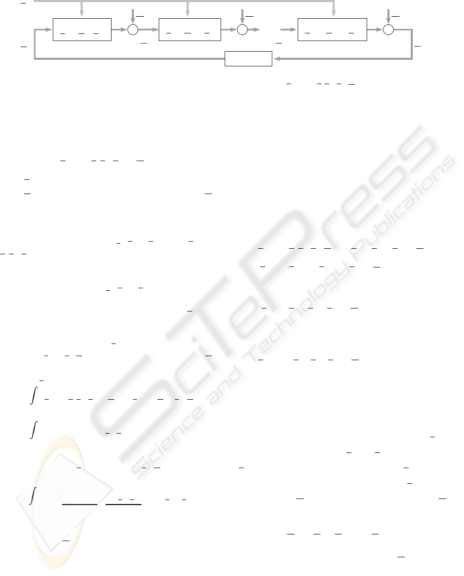
Figure 1: Modularization of the vector valued system x

k+1.

= a

3.2 Vector-Valued Systems

Now we consider the vector-valued system

k+1

= a

) + w

, (8)

with x

k+1

= [x

k+1,1

k+1,2

,. . . ,x

k+1,d

]

∈ R

and

noise w

= [w

k,1

k,2

,. . . ,w

k,d

]

∈ R

. Assuming w

to be white and stationary (but not necessarily Gaus-

sian or zero-mean), with mutually stochastically in-

dependent elements w

k, j

, approximating the corre-

sponding transition density

k+1

) =

k+1

−

)) can be reduced to the scalar system case.

Theorem 1 (Composed Transition Density)

The transition density

k+1

) of system (8)

is composed of separate transition densities of the

scalar systems a

(· ), j = 1,2,. . . ,d, where a

(· ) =

(· ), a

(· ), . ..,a

(· )]

PROOF. Marginalizing

k+1

) from the joint density

function

k+1

) and separating the elements of w

leads to

k+1

)

δ(x

k+1

−a

)−w

)

)dx

∏

j=1

δ(x

k+1, j

− a

) − w

k, j

)

∏

j=1

k, j

)dx

∏

j=1



k+1, j

− a

)



{z }

separate transition densities

)dx

As a result of the mutually stochastically independence of

the elements in w

, the transition density of the vector-

valued system (8) is separated into d transition densities of

d scalar systems. Approximating these lower-dimensional

transition densities is possible with decreased computa-

tional demand (Huber et al., 2006). 

The concept of modularization, introduced in the

following section, beneﬁts strongly from the result

obtained in Theorem 1.

3.3 Concept of Modularization

For our proposed NMPC framework, we assume that

the nonlinear system is corrupted by element-wise ad-

ditive noise. Incorporating this speciﬁc noise struc-

ture, the previously stated closed-form prediction step

can indirectly be utilized for system (1). Similar to

Rao-Blackwellised particle ﬁlters (de Freitas, 2002),

we can reduce the system in (1) to a set of less com-

plex subsystems with a form according to (8),

k+1

= a

) = a

(m)

) + w

(m)

= a

(m−1)

) + w

(m−1)

(2)

= a

(1)

) + w

(1)

We name this approach modularization, where the

subsystems

(i+1)

= a

(i)

) + w

(i)

, for i = 1, ...,m

correspond to transition densities, that can be approx-

imated according to Section 3.1 and 3.2. Since these

subsystems are less complex than the overall sys-

tem (1), approximating transition densities is also less

complex. Furthermore, a nested prediction can be

performed to obtain the predicted density f

k+1

see Fig. 1. Starting with x

(1)

= x

, each subsystem

(i)

(· ) receives an auxiliary system state x

(i)

and gen-

erates an auxiliary predicted system state x

(i+1)

The noise w

is separated into its subvectors w

(i)

according to

= [w

(1)

(2)

,. . . ,w

(m)

]

in case that the single noise subvectors w

(i)

are mutu-

ally independent.

Example System: Modularization

The system model (2) describing the mobile robot can be

modularized into the subsystems

(2)

= sin(α

) + w

A CLOSED-FORM MODEL PREDICTIVE CONTROL FRAMEWORK FOR NONLINEAR NOISE-CORRUPTED

SYSTEMS

and

k+1

= x

+ v· T · x

(2)

k+1

= α

+ u

+ w

The auxiliary system state x

(2)

is stochastically dependent

on α

. We omitted this dependence in further investigations

of the example system for simplicity.

Please note that there are typically stochastic de-

pendencies between several auxiliary system states.

To consider this fact, the relevant auxiliary system

states have to be augmented to conserve the depen-

dencies. Thus, the dimensions of these auxiliary

states need not all to be equal.

4 COST FUNCTIONS

In this section, two possibilities to model cost func-

tions, the well known quadratic deviation and a novel

approach employing Gaussian mixture cost functions,

are presented. Exploiting the fact that the predicted

state variables are, as explained in the previous sec-

tion, described by Gaussian mixture densities, the

necessary evaluation of the expected values in (4) can

be calculated efﬁciently in closed-form for both op-

tions.

In the following, cumulative value functions ac-

cording to (5) are considered, where g

) de-

notes a step cost within the horizon and g

) a cost

depending on the terminal state at the end of the hori-

zon. The value function J

) is the minimal cost for

the next N steps of the system, starting at state x

plus

the terminal cost g

For simplicity, step costs that are additively de-

composable according to

) = g

) + g

)

are considered, although the proposed framework is

not limited to this case.

4.1 Quadratic Cost

One of the most popular cost functions is the

quadratic deviation from a target value ˇx

or ˇu accord-

ing to

) = (x

− ˇx

)

− ˇx

) .

As in our framework the probability density func-

tion of the state x

is given by an axis-aligned Gaus-

sian mixture f

) with L components, the calcula-

tion of E

)}, which is necessary to compute

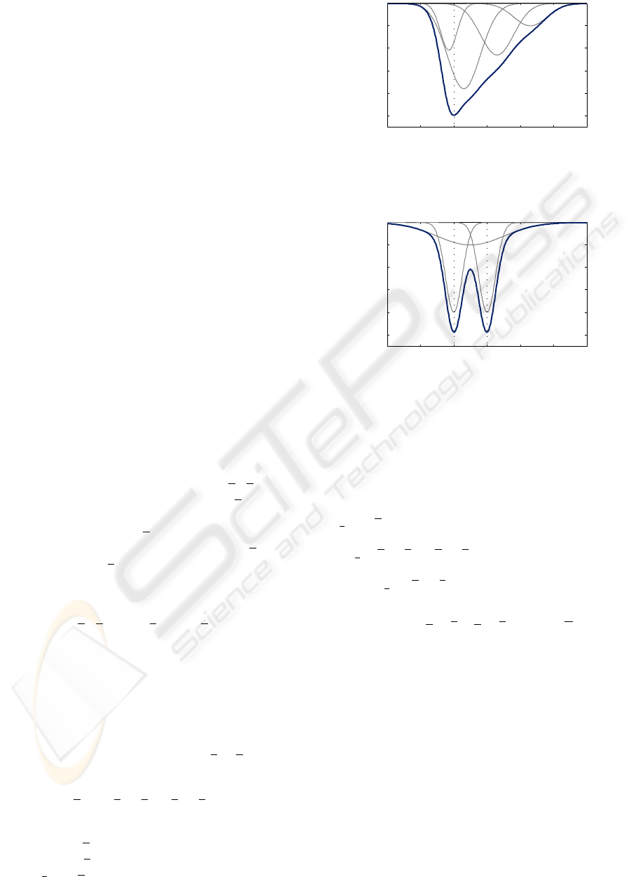
−2 0 2 4 6 8 10

−1

−0.8

−0.6

−0.4

−0.2

→

Figure 2: Asymmetric cost function consisting of four com-

ponents (gray) with a minimum at ˇx

= 2.

−2 0 2 4 6 8 10

−1

−0.8

−0.6

−0.4

−0.2

→

Figure 3: Multimodal cost function consisting of three com-

ponents (gray) with minima at ˇx

= 2, ˇx

= 4.

(4), can be performed analytically as it can be inter-

preted as the sum over shifted and dimension-wise

calculated second-order moments

)}

= E

{(x

− ˇx

)

− ˇx

)}

= trace E

{(x

− ˇx

)}

= trace

∑

i=1



(µ

− ˇx

)(µ

− ˇx

)

+ diag(σ

)



employing E

x} =

∑

i=1

(µ

+ σ

Example System: Quadratic Cost

If the robot is intended to move parallel along the wall, the

negative quadratic deviation of the angle α

with respect to

the wall, i.e., g

(α

) = (α

−α

Wall

)

is a suitable cost func-

tion.

4.2 Gaussian Mixture Cost

A very versatile description of the cost function can

be realized if Gaussian mixtures are employed. In this

case, arbitrary cost functions can be realized due to

the Gaussian mixtures’ universal approximation prop-

erty (Maz’ya and Schmidt, 1996). Obviously, in this

ICINCO 2007 - International Conference on Informatics in Control, Automation and Robotics

case the Gaussian mixtures may have arbitrary param-

eters, e.g. negative weights ω.

Example System: Gaussian Mixture Cost Function

In case the robot is intended to move at a certain optimal

distance to the wall (e.g. ˇx

= 2, with x

Wall

= 0), where

being closer to the wall is considered less desirable than

being farther away, this can, e.g. be modeled with a cost

function as depicted in Fig. 2. If two different distances are

considered equally optimal, this can be modeled with a cost

function as depicted in Fig. 3.

Please note that assigning rewards to a state is

equivalent to assigning negative costs, which leads

to the depicted negative cost functions in Fig. 2 and

Fig. 3.

Here, the calculation of the expected value

)}, which is necessary for the calculation

of (4), can also be performed analytically

)}

)· g

)dx

∑

i=1

N (x

− µ

;diag(σ

)

∑

j=1

N (x

− µ

;diag(σ

)

)dx

∑

i=1

∑

j=1

N (x

− µ

;diag(σ

)

)dx

{z }

with

= ω

N (µ

− µ

;diag(σ

)

+ diag(σ

)

) ,

where f

) denotes the L-component Gaussian

mixture probability density function of the system

state (7) and g

) the cost function, which is a Gaus-

sian mixture with M components.

4.3 Input Dependent Part

The input dependent part of the cost function g

)

can either be modeled similar to the procedures de-

scribed above or with a lookup-table since there is just

a ﬁnite number of discrete u

Using the efﬁcient state prediction presented in

Section 3 together with the value function representa-

tions presented above, (4) can be solved analytically

for a ﬁnite set of control inputs. Thus, an efﬁcient

closed-form solution for the optimal control problem

within NMPC is available. Its capabilities will be il-

lustrated by simulations in the next section.

5 SIMULATIONS

Based on the above example scenario, several simula-

tions are conducted to illustrate the modeling capabil-

ities of the proposed framework as well as to illustrate

the beneﬁts that can be gained by the direct consid-

eration of noise in the optimal control optimization.

The considered system is given by (2) and (3), with

v· T = 1 and u

∈ {−0.2,−0.1, 0, 0.1, 0.2}. The con-

sidered noise inﬂuences on the system w

and w

are

zero-mean white Gaussian noise with standard devia-

tion σ

= 0.5 and σ

= 0.05 ≈ 2.9

◦

respectively. The

measurement noise is also zero-mean white Gaus-

sian noise with standard deviation σ

= 0.5 and σ

0.1 ≈ 5.7

◦

. All simulations are performed for a N = 4

step prediction horizon, with a value function accord-

ing to (5), where g

k+N

) is the function depicted in

Fig. 2 and g

) = g

k+N

) ∀n. In addition, the

modularization is employed as described above.

To evaluate the beneﬁts of the proposed NMPC

framework, three different kind of simulations are

performed:

Calculation of the input without noise considera-

tion (deterministic NMPC):

The deterministic control is calculated as a bench-

mark neglecting the noise inﬂuence.

Direct calculation of the optimal input considering

all noise inﬂuences (stochastic NMPC):

The direct calculation of the optimal input with con-

sideration of the noise is performed using the tech-

niques presented in the previous sections. Thus, it is

possible to execute all calculations analytically with-

out the need for any numerical methods. Still, this

approach has the drawback that the computational de-

mand for the optimal control problem increases expo-

nentially with the length of the horizon N. Thus, this

approach is suitable for short horizons only.

Calculation of the optimal input with a value

function approximation scheme and Dynamic Pro-

gramming (stochastic NMPC with Dynamic Pro-

gramming):

In order to be able to use the framework efﬁciently

also for long prediction horizons, it is necessary to

employ Dynamic Programming (DP). Unfortunately,

this is not directly possible, as no closed-form so-

lution for the value function J

is available. One

easy but either not very accurate or computation-

ally demanding solution would be to discretize the

state space. More advanced solutions can be found

by value function approximation (Bertsekas, 2000).

For the simulations, an especially well-suited case of

A CLOSED-FORM MODEL PREDICTIVE CONTROL FRAMEWORK FOR NONLINEAR NOISE-CORRUPTED

SYSTEMS

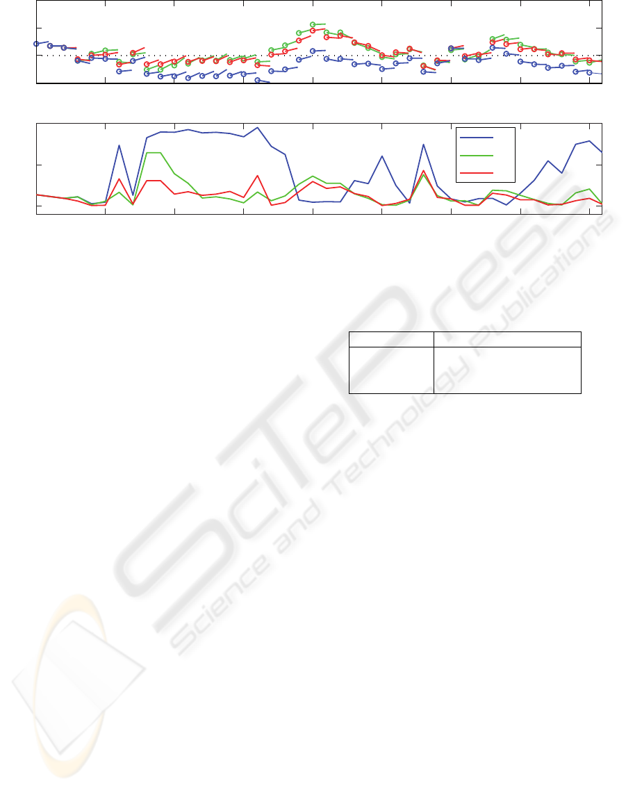
0 5 10 15 20 25 30 35 40

k →

→

(b) Cost per step.

(a) Position and orientation.

0 5 10 15 20 25 30 35 40

−1

−0.5

k →

→

det

Figure 4: First 40 steps of a simulation (red solid line: stochastic NMPC, green dotted line: stochastic NMPC with DP, blue

dashed line: deterministic NMPC).

value function approximation is employed that has

been described by (Nikovski and Brand, 2003). Here,

the state space is discretized by covering it with a

ﬁnite set of Gaussians with ﬁxed means and covari-

ances. Then weights, i.e., scaling factors, are selected

in such a way that the approximate and the true value

function coincide at the means of every Gaussian. Us-

ing these approximate value functions together with

the techniques described above, again all calculations

can be executed analytically. In contrast to the di-

rect calculation, now the computational demand in-

creases only linearly with the length of the predic-

tion horizon but quadratically in the number of Gaus-

sians used to approximate the value function. Here,

the value functions are approximated by a total of 833

Gaussians equally spaced over the state space within

( ˆx

) ∈ Ω := [−2, 10] × [−2,2].

For each simulation run, a particular noise realiza-

tion is used that is applied to the different controllers.

In Fig. 4(a), the ﬁrst 40 steps of a simulation run are

shown. The distance to the wall x

is depicted by the

position of the circles, the orientation α

by the orien-

tation of the arrows. Besides that the system is heav-

ily inﬂuenced by noise, it can be clearly seen that the

robot under deterministic control behaves very differ-

ently from the other two. The deterministic controller

just tries to move the robot to the minimum of the

cost function at ˇx

= 2 and totally neglects the asym-

metry of the cost function. The stochastic controllers

lead to a larger distance to the wall, as they consider

the noise affecting the system in conjunction with the

non-symmetric cost function.

In Fig. 4(b), the evaluation of the cost function for

each step is shown. As expected, both stochastic con-

trollers perform much better, i.e., they generate less

Table 1: Simulation Results.

controller average cost

deterministic -0.6595 (100.00%)

stochastic -0.7299 (110.66%)

stochastic DP -0.6824 (103.48%)

cost, than the deterministic one. This ﬁnding has been

validated by a series of 100 Monte Carlo simulations

with different noise realizations and initial values.

The uniformly distributed initial values are sampled

from the interval x

∈ [0,8] and α

∈ [−π/4,π/4].

In Table 1, the average step costs of the 100 simu-

lations with 40 steps each are shown. To facilitate the

comparison, also normalized average step costs are

given. Here, it can be seen that the stochastic con-

troller outperforms the deterministic one by over 10%

in terms of cost. In 82% of the runs, the stochastic

controller gives overall better results than the deter-

ministic one. By employing dynamic programming

together with value function approximation the bene-

ﬁts are reduced. Here, the deterministic controller is

only outperformed by approximately 3.5%. The anal-

ysis of the individual simulations leads to the conclu-

sion that the control quality signiﬁcantly degrades in

case the robot attains a state which is less well ap-

proximated by the value function approximation as it

lies outside Ω. Still, the dynamic programming ap-

proach produced better results than the deterministic

approach in 69% of the runs. These ﬁndings illustrate

the need for advanced value function approximation

techniques in order to gain the very good control per-

formance of the direct stochastic controller together

with the efﬁcient calculation of the DP approach.

ICINCO 2007 - International Conference on Informatics in Control, Automation and Robotics

6 CONCLUSIONS

A novel framework for closed-form Nonlinear Model

Predictive Control (NMPC) for continuous state space

and a ﬁnite set of control inputs has been presented

that directly incorporates the noise inﬂuence in the

corresponding optimal control problem. By using the

proposed state prediction methods, which are based

on transition density approximation by Gaussian mix-

ture densities and complexity reduction techniques,

the otherwise not analytically solvable state predic-

tion of nonlinear noise affected systems can be per-

formed in an efﬁcient closed-form manner. Another

very important aspect of NMPC is the modeling of the

cost function. The proposed methods also use Gaus-

sian mixtures, which leads to a level of ﬂexibility far

beyond the traditional representations. By employing

the same representation for both the predicted proba-

bility density functions and the cost functions, NMPC

is solvable in closed-form for nonlinear systems with

consideration of noise inﬂuences. The effectiveness

of the presented framework and the importance of

the consideration of noise in the controller have been

shown in simulations of a two-wheeled differential-

drive robot following a speciﬁed trajectory.

Future research is intended to address various top-

ics. One is the optimization of the value function ap-

proximation by abandoning a ﬁxed grid in order to in-

crease performance and accuracy. An additional im-

portant task will be the consideration of stability as-

pects, especially in cases of approximated value func-

tions. This can, e.g. be tackled by the use of bounding

techniques for the approximation error (Lincoln and

Rantzer, 2006). Another interesting extension will be

the incorporation of effects of inhomogeneous noise,

i.e., noise with state and/or input dependent noise lev-

els. Together with the incorporation of nonlinear ﬁl-

tering techniques this is expected to increase the con-

trol quality even more.

Besides the addition of new features to the frame-

work, also the extension to new application ﬁelds is

intended. Of special interest is the extension of Model

Predicted Control to the related emerging ﬁeld of

Model Predictive Sensor Scheduling (He and Chong,

2004), which is of special importance, e.g. in sensor-

actuator-networks.

REFERENCES

Bertsekas, D. P. (2000). Dynamic Programming and Op-

timal Control. Athena Scientiﬁc, Belmont, Mas-

sachusetts, U.S.A., 2nd edition.

Camacho, E. F. and Bordons, C. (2004). Model Predictive

Control. Springer-Verlag London Ltd., 2 edition.

Deisenroth, M. P., Ohtsuka, T., Weissel, F., Brunn, D., and

Hanebeck., U. D. (2006). Finite-Horizon Optimal

State Feedback Control of Nonlinear Stochastic Sys-

tems Based on a Minimum Principle. In Proc. of the

IEEE Int. Conf. on Multisensor Fusion and Integra-

tion for Intelligent Systems, pages 371–376.

Findeisen, R. and Allg

ower, F. (2002). An Introduction to

Nonlinear Model Predictive Control. In Scherer, C.

and Schumacher, J., editors, Summerschool on ”The

Impact of Optimization in Control”, Dutch Institute of

Systems and Control (DISC), pages 3.1–3.45.

de Freitas, N. (2002). Rao-Blackwellised Particle Filtering

for Fault Diagnosis. In IEEE Aerospace Conference

Proceedings, volume 4, pages 1767–1772.

He, Y. and Chong, E. K. P. (2004). Sensor Scheduling for

Target Tracking in Sensor Networks. In Proceedings

of the 43rd IEEE Conference on Decision and Control,

volume 1, pages 743–748.

Huber, M., Brunn, D., and Hanebeck, U. D. (2006). Closed-

Form Prediction of Nonlinear Dynamic Systems by

Means of Gaussian Mixture Approximation of the

Transition Density. In Proc. of the IEEE Int. Conf.

on Multisensor Fusion and Integration for Intelligent

Systems, pages 98–103.

Kalman, R. E. (1960). A new Approach to Linear Filtering

and Prediction Problems. Transactions of the ASME,

Journal of Basic Engineering, (82):35–45.

Lee, J. H. and Ricker, N. L. (1994). Extended Kalman Filter

Based Nonlinear Model Predictive Control. In Indus-

trial & Engineering Chemistry Research, pages 1530–

1541. ACS.

Lincoln, B. and Rantzer, A. (2006). Relaxing Dynamic Pro-

gramming. IEEE Transactions on Automatic Control,

51(8):1249–1260.

Maz’ya, V. and Schmidt, G. (1996). On Approximate Ap-

proximations using Gaussian Kernels. IMA Journal of

Numerical Analysis, 16(1):13–29.

Nikovski, D. and Brand, M. (2003). Non-Linear Stochas-

tic Control in Continuous State Spaces by Exact In-

tegration in Bellman’s Equations. In Proc. of the

2003 International Conf. on Automated Planning and

Scheduling, pages 91–95.

Ohtsuka, T. (2003). A Continuation/GMRES Method for

Fast Computation of Nonlinear Receding Horizon

Control. Automatica, 40(4):563–574.

Qin, S. J. and Badgewell, T. A. (1997). An Overview of In-

dustrial Model Predictive Control Technology. Chem-

ical Process Control, 93:232–256.

Schweppe, F. C. (1973). Uncertain Dynamic Systems.

Prentice-Hall.

A CLOSED-FORM MODEL PREDICTIVE CONTROL FRAMEWORK FOR NONLINEAR NOISE-CORRUPTED

SYSTEMS