
ESCAPE LANES NAVIGATOR
To Control “RAOUL” Autonomous Mobile Robot
Nicolas Morette, Cyril Novales and Laurence Josserand
Laboratoire Vision & Robotique,Orleans Universiy,63 avenue de Lattres de Tassigny,18020 Bourges cedex, France
Keywords: Robotics, Mobile robots, Autonomous robot, Navigation, Escape lanes.
Abstract: This paper presents a navigation method to control autonomous mobile robots :
the escapes lanes, applied
to RAOUL mobile system. First, the formalism is introduced to model an automated system, and then is
applied to a mobile robot. Then, this formalism is used to describe the escape lanes navigation method, and
is applied to our RAOUL mobile robot. Finally, implementation results simulations validate the concept.
1 INTRODUCTION
In the autonomous robotics field, the navigator is
defined as a module whose purpose is to find a
relevant trajectory for a robot within its local
surrounding area. The navigator has to deal with
various robot constraints (such as kinematic
constraints or saturations), and has to find a
trajectory which avoid collisions with static or
mobile obstacles. The trajectory proposed by the
navigator respecting these constraints is followed by
the robot using the pilot and servoings modules.
There are various methods to generate a path for
an
autonomous mobile robot in an unknown
environment. Artificial potential fields methods
(
Agirrebeitia, 2005) generate a path along the weakest
potential gradient, in a potential fields map where
obstacles are associated with strong potentials. The
neural networks methods define a succession of
nodes in a neural network map of the robot
environment (Lebedev, 2005). Fuzzy Logic methods
define a set of logic rules and can drive a robot to
move safely in its environment (Xu, 1999).
However, according to our definition, a
n
avigation method is a complement to this kind of
approach (called path planning methods), whose
purpose is to find a trajectory in order to follow a
path generated by a path planning method under
local constraints. Moreover, a navigation method has
to generate smooth trajectories.
Two kinds of trajectory generation methods are
i
dentified: those using an inverse model of the robot,
and those using a direct model. Among the first
ones, the flat output method controls the robot in
order to follow a calculated trajectory (Fraisse,
2002). (Munoz, 1994) have parametered B-splines
methods to determine a time parametered trajectory
for the robot. Among the second ones (Belker, 2002)
used an hybrid neural networks method to project
acceptable trajectories for the robot in a local neural
network map. In this paper, another direct model
method based on escape lanes (Novales, 1994) is
developed to project acceptable trajectories for the
robot in its local environment.
2 MODEL OF THE ROBOT
Lots of mobile robot navigation methods are based
on inverse model: the robot desired trajectory is
given by the inverse model, which delivers the
articular set points for the servoings. Due to the
mechanical design, sometimes there is no solution
(non-holonomy). Moreover, if the robot evolves in a
constrained environment, cartesian constraints must
be expressed in the robot articular space.
We have chosen to use a direct model of the
m
obile robot to control it. There is always a solution,
and the environmental constraints can be expressed
directly in the cartesian space. As a consequence, we
need to use a global model of the robot and of its
environment, which allows to project all the
admissible trajectories in a near future (a time
horizon of few seconds).
45
Morette N., Novales C. and Josserand L. (2007).
ESCAPE LANES NAVIGATOR - To Control “RAOUL” Autonomous Mobile Robot.
In Proceedings of the Fourth International Conference on Informatics in Control, Automation and Robotics, pages 45-52
DOI: 10.5220/0001625600450052
Copyright
c
SciTePress
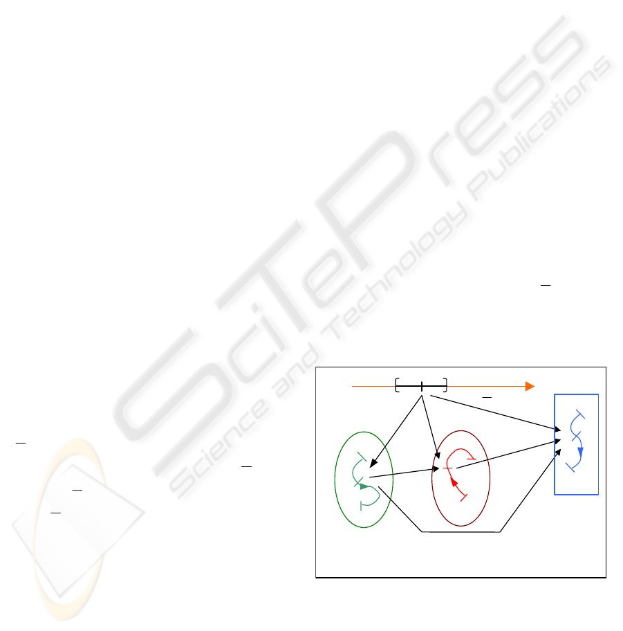
2.1 Formalism of an Automated
System
Based on the formalism developed by Sontag
(
Sontag, 1990), a mobile robot can be modeled with
spaces and functions defined as follows (Figure 1):
),,,,,( hUt Ψ=Σ
ϕ
χ
(1)
where t is the time space,
U is the input space of the system; u are the
vectors of this input space,
χ is the state space of the system; X are the
vectors of this state space,
Ψ is the output space of the system; Y are the
vectors of this output space,
ϕ is the state function which gives a current state
vector X
a
(at time t
a
) knowing the initial time t
0
, the
current time t
a
, the initial state X
0
and the input
function ω (defined later).
h is the output function which gives the current
output vector Y
a
(at time t
a
) knowing the current
time t
a
and state X
a
.
The input function ω associates an input vector
u
a
to the current time t
a
( ω(t
a
) = u
a
).
The transfer function λ associates the current
output vector Y
a
to the current input vector U
a
at
time t
a
and the input function ω (usually it is
hD
ϕ
).
Sontag defines simplified functions ξ(t) and λ(t)
associating either a state vector or an output vector
directly from the current time.
ξ(t), the simplified state function, makes it
possible to define state X
a
of the system time t
a
: ξ(t
a
)
= X
a
. Note that ξ is the image of ω by ϕ in the state
space:
),,,()(
00
ω
ϕ
ξ
Xttt
aa
=
λ
(t) is the simplified exit function which gives
the exit vector Y
a
of the system at time t
a
:
λ
(t
a
) =
Y
a
. Note that
λ
is the image of ξ by h in the space
of exit ψ:
)()(
aa
tht
ξλ
D=
.
2.2 Spaces Specification
In the case of a mobile robot, the contents of the
vectors associated with each space are specified, in
order to introduce our navigation method in section
3.
In the input space U of the robot, vectors
contains set points of the actuator servoings input,
i.e. the articular velocities of the robot:
.
T
n
qqqu ),...,,(
21
=
In the state space χ of the mobile robot, the state
vectors are defined as kinematics values, i.e. the
curvilinear velocities and the rotation velocity of the
mobile robot: .
T
sX ),(
θ
=
The robot output space Ψ is the configuration
space
(Lozano-Perez, 1983), where output vectors are
defined as the coordinates/orientation of the robot:
.
T
yxY ),,(
θ
=
This implies the output function becomes a
differential function and does not depend only on the
current state. The new output function L which gives
the current output vector Y
a
at the current time t
a
depends on the initial time t
0
, on the initial output Y
0
and on the simplified state function ξ.
Our mobile robot is then defined by
),,,,,( LUt
Ψ
=
Σ
ϕ
χ
.
2.3 Definition of a Trajectory
A trajectory Γ of a given system Σ defined on an
interval of time [t
0
, t
0
+ τ] is composed by the
simplified state function ξ and the function of entry
ω defined on the same interval: Γ = (ξ, ω)
nb: the simplified exit function
L
(t) is the
image of the trajectory Γ(t) in the output space.
Typically, it is the “trace on the floor” of the
trajectory of the robot.
t
0
t time
t
a
t
1
ω
(t
a
)
L(t
a
)
ξ
(t
a
)
L(t
0
, Y
0
, t
a
,
ξ
)
ϕ
(t
o
, X
o
,
t
a
,
ω
)
λ
u
1
u
0
u
a
X
o
X
1
X
a
Y
o
U
input space
χ
state space
ψ
output
space
Y
1
Y
a
Figure 1: Automated system
),,,,,( LUt Ψ=Σ
ϕ
χ
.
3 ESCAPE LANES FORMALISM
Similarly to animal strategy, our navigation is based
on direct models. When a mobile robot is considered
ICINCO 2007 - International Conference on Informatics in Control, Automation and Robotics
46
in a given state, we can project in a few seconds
horizon all trajectories that it can perform. These
trajectories can be blended with the environment and
with the motion goal to select the most appropriate
trajectory. These selected trajectories become the
new set points of the mobile robot. In order to give
the ability to the robot to react in real time to its
environment, the process is repeated periodically.
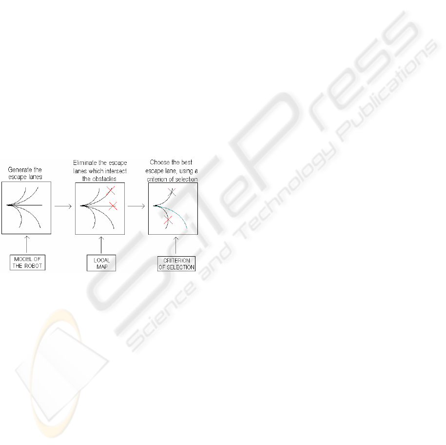
The different steps of the escape lanes method
are to:
- generate all acceptable trajectories Γ to be
performed by the robot (called escape lanes) on a
temporal horizon τ,
- eliminate the blocked escape lanes (e.g.
intersect or pass too close to obstacles),
- choose a free escape lane for the robot, using a
selection criterion.
The strong point of this method is that it uses
only the robot direct model, the inverse function of
ϕ does not need to be defined.
The whole operation is reiterated periodically
and is represented on
Figure 2.
Figure 2: Escape lanes principle.
3.1 Acceptable Trajectories by the
Robot and Escape Lanes
An input function ω is acceptable by the robot on an
interval [t
0
, t
0
+ τ] if it respects the following
constraints:
-constraints corresponding to the direct
kinematics model of the robot, i.e. its possibilities of
movements (kinematics constraints),
-constraints of actuators saturation,
-constraints on the dynamics of the actuators
(maximum accelerations, saturations…)
Ω[t
0
, t
0
+ τ] is called the entire set of the
acceptable input functions on the interval [t
0
, t
0
+ τ] :
[]
{
[]
}
acceptablettUtt
ω
τ
ω
τ
/,,
0000
+
∈=+Ω
(2)
Λ[t
0
, t
0
+ τ] is called the set of the acceptable
trajectories by the robot on the interval [t
0
, t
0
+ τ]. It
corresponds to the set of trajectories associated with
the input function ω є Ω[t
0
, t
0
+ τ]. Λ[t
0
, t
0
+ τ] is also
called the escape lanes of the robot at time t
0
and on
the temporal horizon τ.
[
]
{
[
}
]
τ
ω
ω
ξ
τ
+Ω∈
=
Γ
=
+
Λ
0000
,/),(, tttt
(3)
3.2 Elimination of the Blocked Escape
Lanes
The following stage consists in comparing the image
of each trajectory Γ є Λ in the output space Ψ to the
obstacles map called Θ. This map can be displayed
in several forms, but must imperatively present the
obstacles position with respect to the robot. Using
the elimination criterion C
el
, the ensemble of the free
escape lanes Λ
L
is determinated by:
{
[
}
τλωξ
+Λ∈Γ=Θ=Γ=Λ
Γ 00
,,0),(/),( ttC
elL
]
(4)
Escape lanes which intersect the obstacles or
pass too close to them are eliminated (C
el
≠ 0),
according to C
el
. The remaining escape lanes
constitute the free escape lanes set Λ
L
.
By association, the ensemble of the free
acceptable input functions Ω
L
can be defined as the
entire set of the input functions ω which correspond
to the free escape lanes Λ
L
.
{
}
LL
Λ∈
Γ
Ω
∈
=
Ω
,/
ω
(5)
3.3 Selection of the Best Free Escape
Lane
The last stage consists in determining the best
escape lane among Λ
L
to reach a target ε provided
by the higher control level (i.e. the path planner).
To select the best free escape lane a criterion
C
choice
, is applied to quantify the relevance of each
free escape lane to achieve this goal. The selected
escape lane is associated to the optimal value of the
criterion, and is called Γ
chosen
. The corresponding
function of entry is called ω
chosen
, and is sent to the
lower control level (i.e. the pilot).
{
}
Lchoicechosen
optimalC Λ∈ΓΓ=Γ=Γ ,),(/),(
εωξ
(6)
{
}
L
chosenLchosen
Γ=
Γ
Ω
∈
=
/
ω
ω
(7)
ESCAPE LANES NAVIGATOR - To Control “RAOUL” Autonomous Mobile Robot
47
3.4 Discussion on Criteria
The choice of the C
choice
and C
el
criteria depends on
the application to be carried out by the robot. For an
exploration mission, when the purpose of the robot
is to chart the surrounding area, a severe criterion of
elimination C
el
has to be established to make sure
that the robot passes at a safe distance away from
obstacles (the obstacles positions are known, but
their shapes and volumes are not). A criterion of
selection C
choice
that supports the most efficient
trajectories in term of energy may be used.
On the other hand, when considering missions of
an industrial type, the robot velocity is favored, and
thus the C
choice
criterion must support the fastest
trajectories (at the expense of the energy
consumption). Thus, these criteria must be adapted
to the situation (mission and kind of environment).
The input function corresponding to the selected
trajectory (ω
chosen
) is actually applied to the robot.
Indeed the complete operation (from the generation
of escape lanes of the robot to the selected selection
of Γ
chosen
and ω
chosen
), is performed periodically, and
with a period T
e
about ten times smaller τ. Therefore
only a short portion of the Γ
chosen
trajectory is
actually followed by the robot; a new one is
proposed every T
e
.
4 APPLICATION TO RAOUL
MOBILE ROBOT
4.1 Presentation of RAOUL
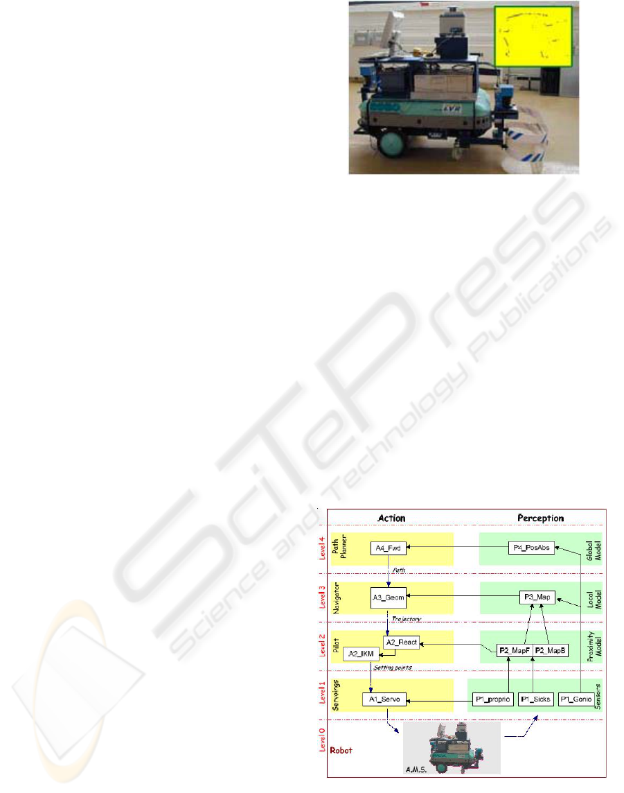
RAOUL (figure 3) is an autonomous mobile robot,
able to run in an unknown environment, finding a
trajectory on its own to avoid collision with static or
mobile obstacles. Raoul is built on a Robuter
platform (Robosoft) with an additional computer
(PC/RTAI-Linux) and exteroceptive sensors: two
Sick telemeters laser (a front one and a rear one) and
one laser goniometer.
Figure 3: The RAOUL robot.
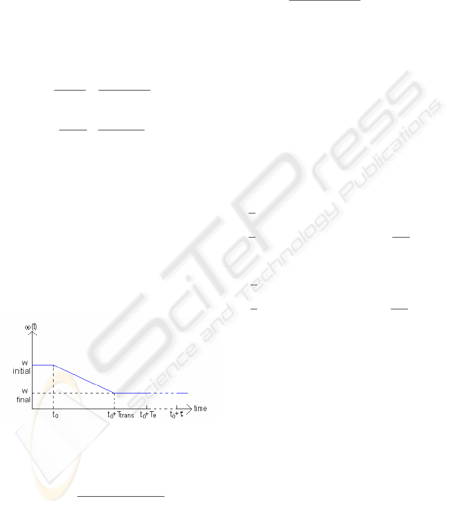
The control architecture (figure 4) is a multi-level
architecture developed by the laboratory of vision
and robotic of the University of Orleans
(Mourioux,
2006). Each level corresponds to a perception/action
loop. Low levels correspond to fast reaction
behaviors and high levels to “intelligent” behaviors.
Level 0 represents the Articulated Mechanical
System (AMS). Level 1 of the architecture
corresponds to the servoings loop using
proprioceptive sensor informations. On level 2, the
“pilot” module performs emergency reactive
decisions, using data from the two laser range
telemeters. The third level, the “navigator”, is in
charge of finding a local trajectory for the robot,
using a local map module
(Canou, 2004). On the
upper level, the “path planner” has the mission to
find a global path for the robot.
Figure 4: the control architecture.
The part developed in this work concern only the
navigation level.
ICINCO 2007 - International Conference on Informatics in Control, Automation and Robotics
48
4.2 Acceptable Trajectories
First the constraints of our system are determined to
define the ensemble of the functions of acceptable
entry Ω on a temporal horizon τ.
RAOUL is a mobile robot with differential
wheels; we assume that the motion is done without
slipless on the ground. According to the
trigonometrical direction for w
1
and w
2
(the rotation
velocity of the two driving wheels) we obtain:
22
1221
RwRwss
s
−
=
+
=
(8)
L
RwRw
L
ss
22
1221
+
=
−
=
θ
(9)
Where s corresponds to the curvilinear distance
traversed by point C, and θ the orientation of the
robot.
The dynamic constraints and saturations depend
on the robot itself and correspond to
.,,,
maxminmin
wwww
x
ma
It is then necessary to choose a family (or a
number finished families) of input functions, that
must be selected according to the robot capacities.
For example, a car-like robot is not controlled the
same way as a robot with differential wheels.
Linear functions are used for RAOUL robot and
are represented on
Figure 5.
Figure 5: Function of entry.
This family of input functions can be expressed
in the following way:
trans
trans
initialfinal
initial
Ttttfor
T
ttww
wtw
+<<
−×−
+=
00
0
)()(
)(
(10)
Under the constraints:
maxmin
maxmin
maxmin
)(
w
T
ww
w
www
www
trans
initialfinal
final
initial
≤
−
≤
≤≤
≤
≤
(11)
From this family of acceptable input functions,
we obtain a family of acceptable trajectories Λ
limited
:
[]
{
}
τ
ξ
+Ω∈
=
Γ
=
Λ
00
,/),( ttww
famillyfamillyLIMITED
(12)
With:
),(
))(),((
21
θξ
s
twtww
T
familly
=
=
(13)
Where:
[]
⎭
⎬
⎫
⎩
⎨
⎧
−
⋅−−−+−⋅=
−⋅=
trans
ififii
T
tt
wwwwww
R
s
twtw
R
s
0
112212
12
()()(
2
))()((
2
(14)
[]
⎭
⎬
⎫
⎩
⎨
⎧
−
⋅−+−++⋅=
+⋅=
trans
ififii
T
tt
wwwwww
R
twtw
R
0
112212
21
()()(
2
))()((
2
θ
θ
(15)
nb: these trajectories are projected starting from
the X
0
state and of the Y
0
output of the robot at time
t
0
.
4.3 Elimination of the Blocked Escape
Lanes
To eliminate the blocked escape lanes a comparison
criterion between Λ
limited
and the map of the
obstacles Θ is proposed.
The local model of the robot environment made
by
(Canou, 2004) is used, built in-line using 2 laser-
range finders. The obstacles map Θ is composed as a
set of segments of known two ends coordinates.
These segments represent the obstacles perimeter in
the local environment of the robot, projected within
the moving plane of the robot.
To determine if an escape lane of Λ
limited
is free
or blocked, the C
el
elimination criterion is used
ESCAPE LANES NAVIGATOR - To Control “RAOUL” Autonomous Mobile Robot
49

between its image λ
i
in Ψ and each obstacle segment
of Θ. C
el
(λ
i
, Θ) = 0 if:
{}
.0)arg(/)( jinmLsgmttdist
ji
∀>+−
λ
(16)
L: maximum distance between the periphery of the
robot and the center C of the axis connecting the two
driving wheels of the robot; L is also called width of
the robot.
dist{
λ
i
(t) / sgmt
j
} is the minimal distance
between λ
i
points and the points belonging to
segment
j
.
Escape lanes that do not verify C
el
(λ
Γ
, Θ) = 0
are eliminated. The ensemble of the remaining
escape lanes is Λ
L / limited
.
4.4 Selection of the Best Free Escape
Lane
Finally a criterion is given to choose the escape lane
to be kept as set point for the robot. The choice of
this criterion takes into account the distance and the
orientation of the robot at the end of the trajectory,
compared to its target ε (provided by the path-
planner).
The criterion is given by:
factytyxtxC
iiichoice
×−++−+=Γ
2
0
2
0
))(())((),(
εε
ττε
(17)
robotetti
tkfact
/arg0
)(1
θτθ
θ
−+×+=
(18)
k
θ
is a positive real fixed empirically by carrying
out simulations and experimentations.
This criterion computes the cartesian distance
from the robot with ε by balancing it with its
orientation compared to ε.
The Λ
L / limited
escape lane which minimizes this
criterion is chosen and called Γ
chosen
. The associated
input function, ω
chosen
, is applied to the robot.
To improve the relevance of the elimination
criterion C
el
, the margin value in the formula (17)
may be adjusted according to the orientation of the
robot with respect to the obstacle (C-obstacles
(Lozano, 1983)).
5 IMPLEMENTATION
Matlab was used to carry out simulations and the
implementation on the robot was made in C
language on Linux RTAI system.
5.1 Discretization of the Input Space
In our case the input space is discretized on 5 by 5
mode, i.e. when the generation of possible
trajectories is carried out, 5x5 = 25 trajectories are
generated corresponding to the 25 possible input
functions ; each one moving towards one of the 25
possible couples (w
1
, w
2
) reached at the end of T
trans
.
The more the space of entry is discretized in a
great number, the greater trajectories number is
possible for our robot at time t
0
. As a consequence
the computation time is higher. It is thus necessary
to find a compromise.
5.2 Generation Off-Line or On-Line of
Λ
Limited
Experimentally, there are two possibilities to carry
out the generation of the possible Λ
limited
. Thos
generation can be performed on line, i.e. while the
robot is moving and just before their application, or
to do it partially off line.
When fully done on line, 5x5=25 trajectories
have to be generated for the robot (or n² if Ω is
discretized by n on n). That is multiplied by the
number of points on each trajectory, i.e. τ divided by
the step of calculation over time. In simulations, a
temporal horizon τ=3s is used for a step of 0.05s, i.e.
a total of 60 points per trajectory and thus 1500
points overall.
Another solution consists in carrying out the
generation of Λ
limited
off line. However, it is then
necessary to generate 5x5 x 5x5 = 625 trajectories.
The trajectories to join the 25 discretized final
couples (w
1
, w
2
) have to be computed, with the 25
possible initial couples as a starting point. It is then
necessary to store all these trajectories during on-
line navigation; the 25 trajectories corresponding to
the initial state of the robot are projected, using the
following transform matrix:
chosen
tttt
y
x
y
x
y
x
Γ+
⎥
⎥
⎥
⎦
⎤
⎢
⎢
⎢
⎣
⎡
•
⎥
⎥
⎥
⎦
⎤
⎢
⎢
⎢
⎣
⎡
−
+
⎥
⎥
⎥
⎦
⎤
⎢
⎢
⎢
⎣
⎡
=
⎥
⎥
⎥
⎦
⎤
⎢
⎢
⎢
⎣
⎡
/
100
0cossin
0sincos
00
θ
θθ
θθ
θθ
(19)
This solution is used when the robot does not
have the necessary power to perform all the
calculations on line. The totality of the generated
trajectories is represented on figure 6.
ICINCO 2007 - International Conference on Informatics in Control, Automation and Robotics
50
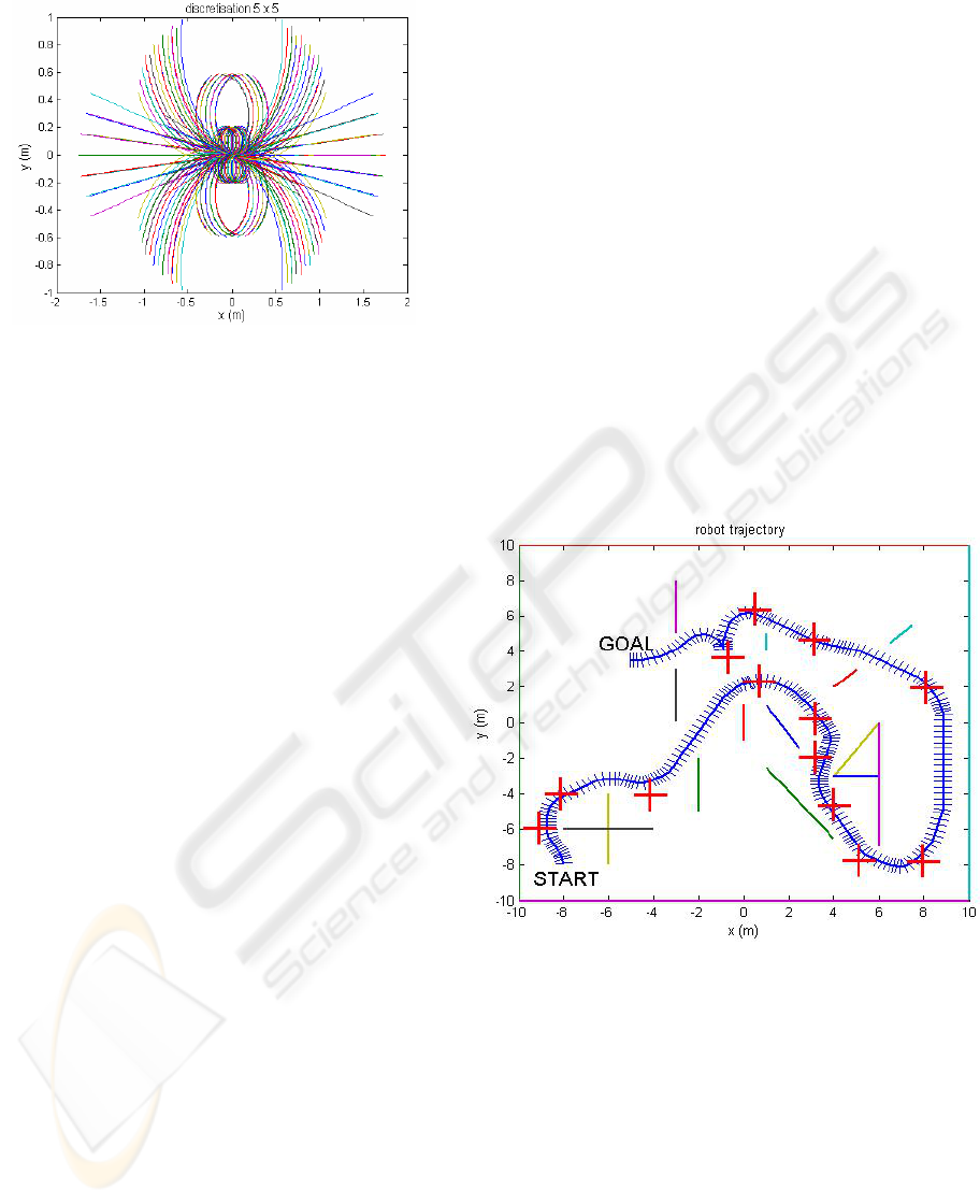
Figure 6: Possible trajectories of the robot stored in
memory.
5.3 Implementation
Experimentally, we are constrained to perform the
navigation calculation one period T
e
ahead of time.
Indeed, calculations for the period [t
0
, t
0
+T
e
] as from
time t
0
since it takes a certain time for calculation
and since the robot continues to move forward
during this time.
The navigation calculation for the period [t
0
,
t
0
+T
e
] must thus be carried out during the period [t
0
-
T
e
, t
0
]. To know the robot output Y at t
0
, we carry
out the approximation which the robot will have
followed exactly the escape lane chosen over the
period [t
0
-T
e
, t
0
], starting from its output Y at the
moment t
0
- T
e
.
[]
00
000
,
/
100
0cossin
0sincos
tTton
T
TtTtt
e
chosene
ee
y
x
y
x
y
x
−
Γ
−−
⎥
⎥
⎥
⎦
⎤
⎢
⎢
⎢
⎣
⎡
•
⎥
⎥
⎥
⎦
⎤
⎢
⎢
⎢
⎣
⎡
−
+
⎥
⎥
⎥
⎦
⎤
⎢
⎢
⎢
⎣
⎡
=
⎥
⎥
⎥
⎦
⎤
⎢
⎢
⎢
⎣
⎡
θ
θθ
θθ
θθ
(20)
6 RESULTS
6.1 Simulation
The simulation program that we have developed is
composed of three parts. The first part calculates and
stores in memory the possible movements of the
robot (off-line generation of Λ
limited
).
The second creates a chart of a virtual
environment in which the robot will navigate. This
environment consists in obstacles viewed as
segments (these segments represent the periphery of
the obstacles in the navigation plan).
The last part corresponds to navigation itself,
and includes the projection stages of the robot
escape lanes, the elimination of the blocked escape
lanes and the choice of the most suitable escape
lane. This part is performed until the virtual robot
reaches a desired localization (beyond a certain
number of loops the program stops). Finally the
program traces the path that the robot carries out on
the chart, and gives the inputs list sent to the robot
with each iteration.
6.2 Results
Figure 7 shows a simulation representing
displacements of the robot using a differential
wheels type model. The robot starts at point
coordinates (-8, -8), and must go to (-5, 4).
Figure 7: Simulation of obtained trajectory.
The trace of the displacements achieved by the
center of the robot is represented in blue, and each
new iteration of the program of navigation is
symbolized by a small feature perpendicular to the
trace. The red crosses represent the points of passage
provided to the navigator.
ESCAPE LANES NAVIGATOR - To Control “RAOUL” Autonomous Mobile Robot
51
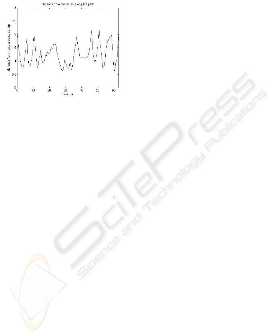
Figure 8: distance robot/obstacle.
The distance between the robot and its nearest
obstacle along the path is represented on figure 8.
We can note that the robot never enters in collision
with the obstacles because the distance from
obstacles is larger than the robot width (50cm).
Moreover in the event of appearance of an
unexpected obstacle, the pilot (i.e. the lower level of
control) has the capacity to perform reflex decisions,
of absolute priority, to avoid this kind of obstacle in
emergency. We can note the great flexibility of the
generated trajectories.
7 CONCLUSION
This study showed that escape lanes is an efficient
navigation method, able to generate fluent moves for
RAOUL autonomous mobile robot. Its strong point
is that it only uses the direct kinematics model of the
robot, ensuring that the robot is actually able to
perform the desired moves. Indeed it's more difficult
to transpose constraints in the input space of the
robot using an inverse model.
However it's only a navigation method, meaning
that it must work cooperatively with a path planner
module, which gives a global path to follow to the
navigator. The purpose of the navigator is to follow
this path as close as possible, under the local
constraints of the environment the robot evolves in.
The next step is to implement this method with a
planner on a Cycab robot, using a GPS for the path
planning module. Cycab is a car-like robot, with
only one mobility degree. This will provide a
stronger non holonomy constraint in the
implementation of the proposed navigation method.
REFERENCES
Agirrebeitia, J., Aviles, R., de BUSTOS, I. F., Ajuria, G.,
June 2005, A new APF strategy for path planning in
environments with obstacles, Mechanism and Machine
Theory, Volume 40, Issue 6, , Pages 645-658
Belker, T., Schulz, D., Intelligent Robots and System,
2002, Local Action Planning for Mobile Robot
Collision Avoidance, IEEE/RSJ International
Conference on Volume 1, 30 Sept.-5 Oct. 2002
Page(s):601 - 606 vol.1
Canou, J., Mourioux, G., Novales, C. Poisson, G., April 26
– May 1
st
2004 , A local map building process for a
reactive navigation of a mobile robot, Proceedings of
IEEE International Conference on Robotics and
Automation, pp4839-4844, New Orleans, USA
Fraisse, P., Gil, A. P., Zapata, R., Perruquetti, W., Divoux,
T., 2002, Stratégie de commande collaborative
réactive pour des réseaux de robots.
Lebedev, D. V., April 2005. The dynamic wave expansion
neural network model for robot motion planning in
time-varying environments, Neural Networks, Volume
18, Issue 3, Pages 267-285.
Lozano-Perez, T., 1983, Spatial Planning: a
Configuration Space Approach, IEEE Transaction and
computers, vol. C-32, no. 2, Fev. 1983.
Novales, C., 1994, Navigation Locale par Lignes de Fuite,
rapport de thèse : Pilotage par actions réflexes et
navigation locale de robots mobiles rapides, chapitre
IV, soutenue le 20 octobre 1994, Pages 87 à 107
Novales, C., Mourioux, G., Poisson, G., April 6,7 2006 , A
multi-level architecture controlling robots from
autonomy to teleoperation, First National Workshop
on Control Architectures of Robots – Montpellier
Munoz, V., Ollero, A., Prado, M., Simon, A., 1994 IEEE
International Conference on 8-13 May 1994,
Mobile
robot trajectory planning with dynamic and kinematic
constraints, Robotics and Automation, 1994.
Proceedings, Page(s):2802 - 2807 vol.4
Sontag, E. D., 1990. Mathematical control Theory –
Deterministic Finite Dimensional Systems, ED-
Spronger-Velag New-York 1990.
Xu, W. L., August 1999, A virtual target approach for
resolving the limit cycle problem in navigation of a
fuzzy behavior-based mobile robot, Institue of
Technology and Institute of Technology and
Engineering, College of Sciences, Massey University,
Palmerston North, New Zealand ; Received 22 June
1998 ; accepted 20 August 1999
ICINCO 2007 - International Conference on Informatics in Control, Automation and Robotics
52
